Building a CT Slice Localizer With Keras

Experienced radiologists can identify the anatomical location of an axial CT slice within a second. They may say the slice is “near the apex of the heart” or “at the C7 vertebrae.” These anatomical landmarks are difficult to describe or detect using manually created features, but neural networks excel at this sort of pattern recognition. Can we create a neural network capable of performing slice localization with similar speed and accuracy to a radiologist?

In this article, we describe:

• how we collected and annotated training data,
• how we trained the algorithm,
• applications of the slice localizer, and
• limitations of the model.

For more background information about deep neural networks, check out our article on building an image classifier with Keras, which details another image classification task solved in a similar but not identical way.

Preparing the training data 🔗

A model requires material to learn from, so our first step is to find data it can train on.

A neural network requires a lot of training. Training a network from scratch requires vast amounts of data and time, even with capable hardware. To speed up the training process and improve our resulting model, we utilize a method called transfer learning, where a model developed for a specific task is used as the base of a model for a related task. In this project, we adapt some of the pre-trained models available through Keras for use in CT slice localization.

Gathering CT datasets 🔗

Even with a pre-trained model, additional input data is needed to train it to handle a new task. We collected numerous sets of CT images containing tens of thousands of individual slices as DICOM files from various open access databases:

• CT Medical Images
• National Biomedical Imaging Archive
• Lung Image Database
• Visible Human Project CT Datasets

With data obtained from different sources, folders and files have no consistent naming scheme. We developed a file organizer to standardize the file structure containing the images, splitting them into nested folders based on attributes of the DICOM files: Patient ID, Study Instance UID, and Series Instance UID. Files were named based on their Instance Number attribute.

Annotating slices 🔗

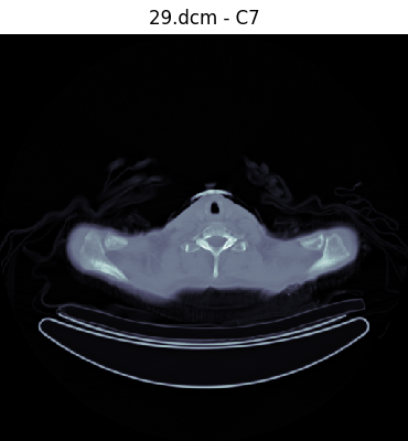
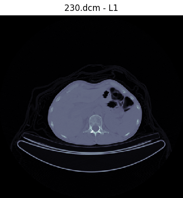
Our network will be trained with supervised learning, a process that uses labeled training data to generate a function that best estimates a relationship between input and expected output. Thus, our first task involves labeling our data. We created a DICOM image viewer and annotation tool that allowed the user to label a slice with an annotation with a single keystroke. We decided to use 12 easily identifiable anatomical landmarks between the head and the femur that are spaced throughout the range.

key_to_label = {
    '`': 'Top of head',
    '1': 'Center of orbit',
    '2': 'C1',
    '3': 'C7',
    '4': 'T1',
    '5': 'Aortic arch',
    '6': 'Bifurcation of trachea',
    '7': 'Right dome of diaphragm',
    '8': 'T12',
    '9': 'L1',
    '0': 'Tip of iliac crest',
    '-': 'Head of femur',
}

Once labels are created, all labels in a dataset are saved as a JSON file mapping the label to the filename:

{
    "C1": "69.dcm",
    "Center of orbit": "103.dcm",
    "C7": "32.dcm",
    "Aortic arch": "5.dcm",
    "T1": "27.dcm"
}

Standardizing the location labels 🔗

We have labeled our slices, but we need a standardized value to represent the slice location. Identical locations in two different CT sets may have different Instance number values and the Slice Thickness attribute can also vary. The offset of values of the Image Position (Patient) attribute varies between scans, so the z-location of a slice at the T1 vertebrae may be -534.8 in one image set and -544.2 in another. This inconsistency makes it difficult to use a DICOM attribute to identify matching locations between two different CT sets. Thus, we map each annotation to a standardized numerical location between 0 and 1 from the head down.

label_to_normalized_location = {
    'Top of head': 0,
    'Center of orbit': .05,
    'C1': .1,
    'C7': .15,
    'T1': .16,
    'Aortic arch': .2,
    'Bifurcation of trachea': .225,
    'Right dome of diaphragm': .275,
    'T12': .325,
    'L1': .35,
    'Tip of iliac crest': .425,
    'Head of femur': .5,
}

With this, all CT slices with the label .2 represent the slice from the set most accurately depicting the aortic arch. However, we have to be able to identify any location within a CT set, not just the annotations. 1-D interpolation is perfect for this, generating normalized location values for each slice dependent on its Image Position (Patient) z-axis value. We want our model to be able to identify locations from head to foot, but our training data doesn’t have enough CT sets with images below the femur, so we use extrapolation to generate values past the lowest annotation. To connect this all together, we use the above dictionary to map each file to its respective normalized location and interpolate the rest of the unlabeled slices, saving the resulting data to a JSON file:

{
    "patient_id/study_iuid/series_iuid/10.dcm": 0.05,
    "patient_id/study_iuid/series_iuid/11.dcm": 0.0625,
    "patient_id/study_iuid/series_iuid/12.dcm": 0.075,
    "patient_id/study_iuid/series_iuid/13.dcm": 0.0875,
    "patient_id/study_iuid/series_iuid/14.dcm": 0.1,
}

Converting the DICOM files 🔗

Now that all the files have a normalized location, the last step in preprocessing the data involves converting the DICOM files into a .npz file format containing data that will be used in training. We want to include the pixel data from each DICOM image, reshaped to fit the pre-trained model’s required input shape, and also its associated normalized location. We also save each image’s Series Instance UID attribute for use in partitioning the data into bins used in training. Since we want all slices from the same CT series to be in the same partition, we will separate them by hashing the Series Instance UID, which will result in identical hash outputs across all images within a single CT dataset.

IMG_SIZE = (256, 256)


if __name__ == '__main__':
    parser = argparse.ArgumentParser()
    parser.add_argument('source_dir', nargs=1, metavar='<dir>',
        help='Directory containing "combined_normalized_locations.json".')
    args = parser.parse_args()
    json_dir = os.path.abspath(args.source_dir[0])
    json_path = os.path.join(json_dir, 'combined_normalized_locations.json')

    with open(json_path, 'r') as f:
        path_to_norm_loc = json.loads(f.read())

    for dcm_rel_path, norm_loc in tqdm(path_to_norm_loc.items()):
        dcm_path = os.path.join(json_dir, dcm_rel_path)
        dcm_file = pydicom.dcmread(dcm_path)
        pixels = dcm_file.pixel_array

        resized_pixels = scipy.misc.imresize(pixels, IMG_SIZE)
        if len(np.shape(resized_pixels)) > 2:
            resized_pixels = resized_pixels[:,:,0]
        # Reshape image to (256, 256, 3)
        # Pre-trained models only accept inputs with three channels
        reshaped_pixels = np.stack([resized_pixels]*3, axis=-1)

        basepath, _ = os.path.splitext(dcm_path)
        dest_path = basepath.replace(os.path.basename(json_dir), 'npz_dataset')
        head, _ = os.path.split(dest_path)
        os.makedirs(head, exist_ok=True)
        np.savez(
            dest_path,
            pixels=reshaped_pixels,
            norm_loc=norm_loc,
            series_instance_UID=dcm_file.SeriesInstanceUID,
            compressed=True
        )

Partitioning the data 🔗

As the last step in preparing for training, we split the dataset into three partitions: training, validation, and testing. We assign each image a partition by hashing its Series Instance UID attribute and calculating the resulting value mod 10 to determine where it goes. In the function below, we put 70% of the data in the training set, 20% in the validation set, and 10% in the testing set and separate each partition into its own directory.

parser = argparse.ArgumentParser()
parser.add_argument('--data-dir', nargs=1, metavar='<dir>',
    help='Directory containing files to sort.')
parser.add_argument('--target-dir', nargs=1, metavar='<dir>',
    help='Directory to save partition directories and sorted files.')
args = parser.parse_args()
data_path = os.path.abspath(args.data_dir[0])
partitions = ['training', 'validation', 'testing']
partition_dirs = dict()
for partition in partitions:
    dir_path = os.path.join(args.target_dir[0], partition)
    partition_dirs[partition] = dir_path
    os.makedirs(dir_path, exist_ok=True)
npz_file_list = [str(path) for path in Path(data_path).glob('**/*.npz')]
for npz_path in tqdm(npz_file_list):
    series_IUID = np.load(npz_path)['series_instance_UID']
    new_file_name = '_'.join([
        str(series_IUID).replace('.', '_'),
        os.path.basename(npz_path)
    ])
    encoded_series_IUID = str(series_IUID).encode('utf-8')
    hash_val = int(hashlib.sha256(encoded_series_IUID).hexdigest(), 16)
    if hash_val % 10 < 7:
        partition = 'training'
    elif 7 <= hash_val % 10 < 9:
        partition = 'validation'
    elif hash_val % 10 == 9:
        partition = 'testing'
    else:
        raise Exception("partition not assigned")
    dest_path = os.path.join(partition_dirs[partition], new_file_name)
    shutil.copy2(npz_path, dest_path)

Training the model 🔗

Detecting a particular anatomical landmark in an image is a classification problem, however, we want to know the axial location of a slice within the body. In other words, since the human body is continuous, we want the algorithm to give us a floating point number describing where the axial slice is localized within the body. Thus, slice localization is better formulated as a regression problem.

Now that we have organized, labeled, and converted our data, we can begin the process of training our model.

Augmenting the training data 🔗

With a relatively small volume of training data, we risk overfitting our model. Overfitting is a phenomena in which a model begins to “memorize” the data instead of learning to generalize, generating a function which too closely fits a set of data points. A good example of “overfitting” would be a student who obtains a copy of an exam and memorizes the question and answer pairs directly instead of learning to solve the questions. To prevent overfitting our model, we augment our data by introducing randomized, realistic modifications with the ImageDataGenerator class to increase the variety of data available to the model.

image_datagen = ImageDataGenerator(
                    rotation_range=15,
                    width_shift_range=.15,
                    height_shift_range=.15,
                    shear_range=.15,
                    zoom_range=.15,
                    horizontal_flip=True,
                    vertical_flip=False,
                )

Customizing a pre-trained model 🔗

Since our training data is limited in volume and we have access to a resource with pre-trained models, we will use transfer learning. This optimization technique can produce in a model that trains faster and performs better than a model trained from scratch. We set up our model with the same process as the one used in the Simpsons example, starting by pulling one of the pre-trained ImageNet models from Keras.

IMG_SIZE = (256, 256)

def get_model(pretrained_model):
    if pretrained_model == 'inception':
        model_base = keras.applications.inception_v3.InceptionV3(
            include_top=False,
            input_shape=(*IMG_SIZE, 3),
            weights='imagenet'
        )
        output = Flatten()(model_base.output)
    elif pretrained_model == 'xception':
        model_base = keras.applications.xception.Xception(
            include_top=False,
            input_shape=(*IMG_SIZE, 3),
            weights='imagenet'
        )
        output = Flatten()(model_base.output)
    elif pretrained_model == 'resnet50':
        model_base = keras.applications.resnet50.ResNet50(
            include_top=False,
            input_shape=(*IMG_SIZE, 3),
            weights='imagenet'
        )
        output = Flatten()(model_base.output)
    elif pretrained_model == 'vgg19':
        model_base = keras.applications.vgg19.VGG19(
            include_top=False, input_shape=(*IMG_SIZE, 3),
            weights='imagenet'
        )
        output = Flatten()(model_base.output)

We remove the top layers of each model by using include_top=False and substitute the final layers with our own. Since our objective is to output a single numerical value instead of a probability distribution, the structure of our model will be slightly different than the one in the Simpsons classifier:

    output = BatchNormalization()(output)
    output = Dropout(0.5)(output)
    output = Dense(128, activation='relu')(output)
    output = BatchNormalization()(output)
    output = Dropout(0.5)(output)
    output = Dense(1, activation='sigmoid')(output)
    model = Model(model_base.input, output)
    for layer in model_base.layers:
        layer.trainable = False
    model.summary(line_length=200)
    model.compile(optimizer='adam',
                  loss='mse')
    return model

In the Simpsons example, one-hot encoding is used to perform “binarization” of categories. The term “one-hot” refers to an encoding system where a group of bits has a single bit with value 1 representing the truth state and the rest with value 0, similar to a multiple choice question with one right answer. Our project, however, will not be using one-hot encoding because the slice localization task is a regression problem that does not involve classification.

Due to this key difference in the type of problem we are tackling, there are a few other differences in how we set our model up. We use a sigmoid activation function for our model’s final layer instead of a softmax activation function, which is more useful for multi-class classification. The sigmoid function works well for our desired output value which resides within a continuous range between 0 and 1.

Additionally, we use a different loss function in our model. The Simpsons classifier utilizes categorical cross-entropy, which is especially effective in multi-class classification problems where labels are one-hot encoded. For a better measure of error in a regression task like ours, we use mean-squared loss. Mean-squared error measures the distance between predicted and expected values within a continuous range. On the other hand, cross-entropy loss measures the differences between discrete probability distributions, and thus is not suitable for our regression task, which involves predicting a real value from a continuous set. To produce the best estimator, we want to minimize the mean-squared error to generate a “line of best fit”.

Once we have our customized final layers, we’ll create a generator to provide data to the model in batches for the training process.

class DataGenerator():
    def __init__(self, data_dir):
        self.data_path = Path(os.path.abspath(data_dir))
        self.partition_to_npz_path = {
            'training': list(),
            'validation': list(),
            'testing': list(),
        }
        partitions = ['training', 'validation', 'testing']
        for partition in partitions:
            part_path = Path(os.path.join(os.path.abspath(data_dir), partition))
            npz_file_list = list(part_path.glob('**/*.npz'))
            for npz_path in npz_file_list:
                self.partition_to_npz_path[partition].append(npz_path)


    def _pair_generator(self, partition, augmented=True):
        while True:
            npz_path = random.choice(self.partition_to_npz_path[partition])
            pixels = np.load(npz_path)['pixels']
            norm_loc = np.load(npz_path)['norm_loc']
            if augmented:
                augmented_pixels = next(image_datagen.flow(np.array([pixels])))[0]
                yield augmented_pixels, norm_loc
            else:
                yield pixels, norm_loc


    def batch_generator(self, partition, batch_size, augmented=True):
        while True:
            data_gen = self._pair_generator(partition, augmented)
            pixels_batch, norm_loc_batch = zip(*[next(data_gen) for _ in range(batch_size)])
            pixels_batch = np.array(pixels_batch)
            norm_loc_batch = np.array(norm_loc_batch)
            yield pixels_batch, norm_loc_batch

Our training interface is the exact same as the one used in the Simpsons classifier, so check out the relevant section for the code and a breakdown.

Applications 🔗

Now that we’ve trained our model, we can use it to perform a number of functions:

Normalized location prediction 🔗

For our most basic function, we can pass an image to our model and have it generate a normalized location value of where it thinks the slice is located:

def predict_location(pixels, model=DEFAULT_MODEL):
    '''
    Predicts the normalized location of a CT image slice
    Input:  pixels = array containing image pixel data
            model = a predictive model
    Output: predicted normalized location
    '''
    pixels = reshape(pixels, model)
    return float(model.predict(np.array([pixels]), batch_size=1))

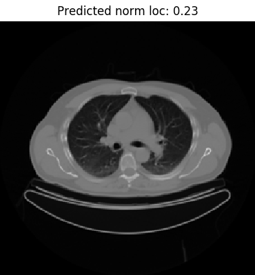
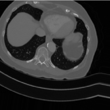
To do a manual check of the model’s predictions, we can reference the label_to_normalized_location dictionary created during training data preparation. As an example, take a look at the image on the left. The predicted value 0.23 suggests that the slice is marginally below the bifurcation of the trachea at the carina level, defined as 0.225. The label seems to be accurate as the image depicts clearly visible left and right primary bronchi.

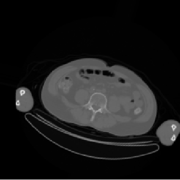
Find matching slices 🔗

A more practical use might be to utilize the model to find matching slices between different CT datasets. Consider the following scenario: a patient comes in for a CT scan and the resulting analysis finds an abnormality in the lung area. If the patient comes back for a follow-up CT a few months later, it would save the radiologist some time by automating the process of finding the slice with the abnormality. In this way, they could perform a comparison of scans over time without having to manually search through each CT dataset for matching images.

def match_files(image_paths, key, tolerance=.01, model=DEFAULT_MODEL):
    '''
    Finds images matching a specified normalized location
    Input:  image_paths = paths of images to check for matches
            key = location value to match
            tolerance = error tolerance for matching
    Output: list of matches in format [path, pixel data, predicted location]
    '''
    matches = list()
    for image_path in tqdm(image_paths, unit='image'):
        pixels = load_pixels(image_path)
        prediction = predict_location(pixels, model)
        error = abs(float(key) - prediction)
        if error <= tolerance:
            tqdm.write('Match found; error = {}'.format(error))
            matches.append((image_path, pixels, prediction))
    return matches

In this function, we take a single key value representing the location target and find all matching images within an error tolerance, returning a list containing each image’s path, pixel data, and predicted location value.

This ability to pull slices with a specific location could be useful in image registration, putting together slices along the z-axis by creating a standardized location value range. In addition, this functionality could be integrated in a larger system. While the slice localizer currently only works with CT images, it could be useful in multi-modal image registration if integrated into a larger system. Additionally, the slice localizer could be used in conjunction with another algorithm that takes the data output as an input for another purpose, such as performing image segmentation on matching images.

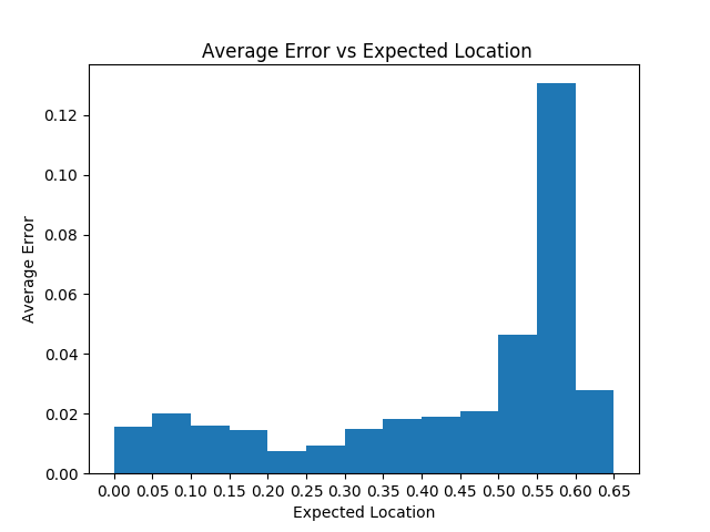
Limitations 🔗

Our slice localizer, while accurate in some areas, does not perform consistently in identifying slices across the body. Since our training data was composed almost entirely of slices between the head and the femur, the model excels at predicting these locations. However, the lack of training data below the femur means that our model is relatively inaccurate at predicting locations of slices below the femur.

To verify this, we’ll run the basic prediction on the entire testing partition and calculate the average error of slices from different areas in the body. The resulting data, plotted below, depicts a significant increase in average error past the .5 mark, which confirms our model’s inability to accurately predict locations below the head of the femur.

When we visualize a plot of predicted locations versus z-axis location , we expect a linear graph. However, we find that linearity is lost when using our model to make predictions past the femur (Z-position > -1050 in the image below):

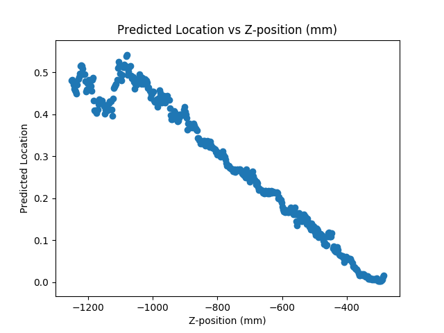
With more training data, especially images below the waist, we could improve the prediction accuracy of our model and reduce the incidence of any overfitting.

Conclusion 🔗

By leveraging Keras’ pre-trained models and customizing the top layers, we have created a library for developing a deep learning model capable of performing CT slice localization with relatively high accuracy. Although our current trained model isn’t as reliable as a professional radiologist, training with more comprehensive data may continue to improve its efficacy. Ultimately, this model can serve as a standalone application or as a base for further functionality involving image processing.