
Want to know how we develop safe, effective, and FDA compliant machine learning algorithms? This article describes how we develop machine learning algorithms, points out common pitfalls, and makes documentation recommendations.
When developing a machine learning or AI algorithm, it’s easy to become overly focused on making the best model possible. While model performance is important, to incorporate the model into a commercial medical device, you’ll need to be able to demonstrate to the FDA that the model is safe and effective. Therefore, it’s critical to thoroughly document the algorithm’s development lineage in your design history file. The process outlined in this article will help you do this. We’ve used it to develop AI algorithms within a recently 510(k)-cleared class-II medical device for one of our clients.
The FDA released its Artificial Intelligence/Machine Learning (AI/ML)-Based Software as a Medical Device (SaMD) Action Plan in January of 2021. In it, they discuss upcoming changes to their approach for regulating ML-based medical devices. The exact details aren’t public, but we suspect following a consistent development process will be part of it.
Focus on process documentation 🔗
Our AI development process includes generating reports that detail the input data, model performance, and model selection process. These reports streamline model development by helping developers recognize and correct some of the most common pitfalls in algorithm development, thereby increasing confidence in the AI/ML algorithm’s safety and efficacy. As a convenient side effect, these reports are a powerful tool when designing a QMS suitable for AI and navigating the FDA clearance process.
Some common pitfalls we have identified are: 🔗
- Laser-focus on chasing higher accuracy metrics and forgetting about the business, clinical, and regulatory context
- Errors in data import and preprocessing
- Clinically unrealistic data augmentation
- Algorithm performance metrics—such as the Dice score—are not a perfect proxy to clinical performance but are treated as such
- Data leakage or improper training/validation splits leads to undetectable overfitting and a false sense of stellar algorithm performance
- Using data that was acquired with non-clinical (research) protocols that are too different from the device’s intended use thereby leading to regulatory risk. 1
- Not being aware of sampling bias in the data thereby leading to regulatory risk. For example, certain age groups may be underrepresented or certain scanner vendors may be overrepresented. 1
These pitfalls can be mitigated by the following reports: 🔗
- Input Verification Report
- Data Augmentation Quality Assurance Report
- Model Performance Report
- Model Comparison Report
Input Verification Report 🔗
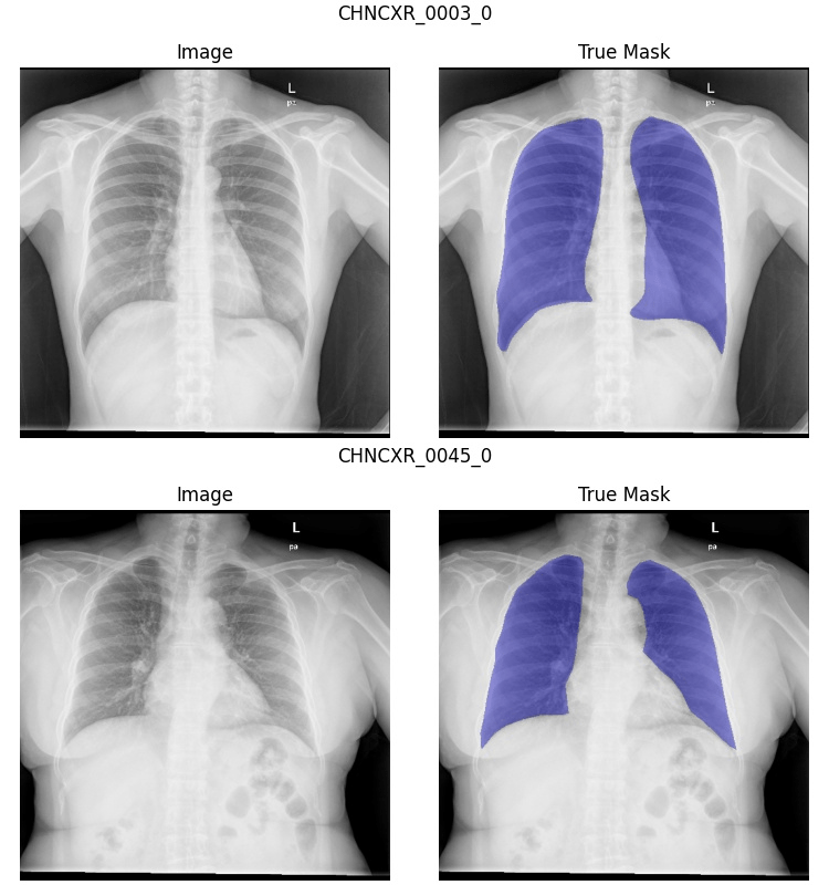
The input verification report should visualize the dataset as close to the model training step as possible. A common source of error can be simple data processing errors. This report is also an excellent way to verify the quality of the data. If the input data is not very accurate to start with, it will be hard to train an accurate model. In other words, “garbage in equals garbage out.”
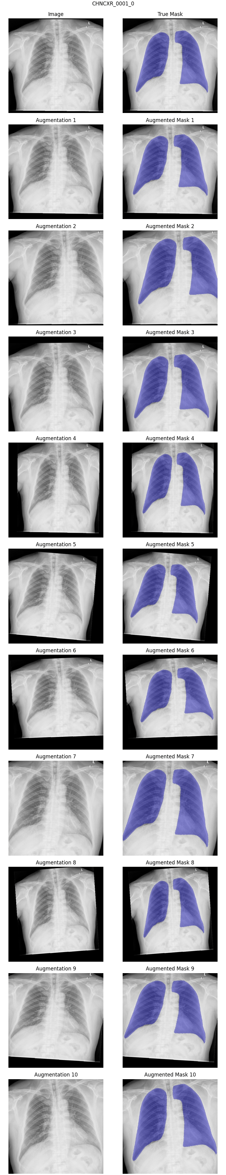
Data Augmentation Quality Assurance (QA) Report 🔗
Data augmentation is a powerful technique that effectively increases the size of your dataset, reducing the risk of overfitting and increasing accuracy. However, going overboard with data augmentation techniques could distort the images beyond realistic boundaries. The data augmentation QA report takes a random sample of the dataset and produces several augmentations of that image and its annotations. This report allows you to confirm the augmented images are still clinically valid and that the annotations—such as segmentations and fiducial markers—are augmented properly.
Model Performance Report 🔗
The model performance report can vary greatly depending on the problem. However, there are four essential properties that this report should have:
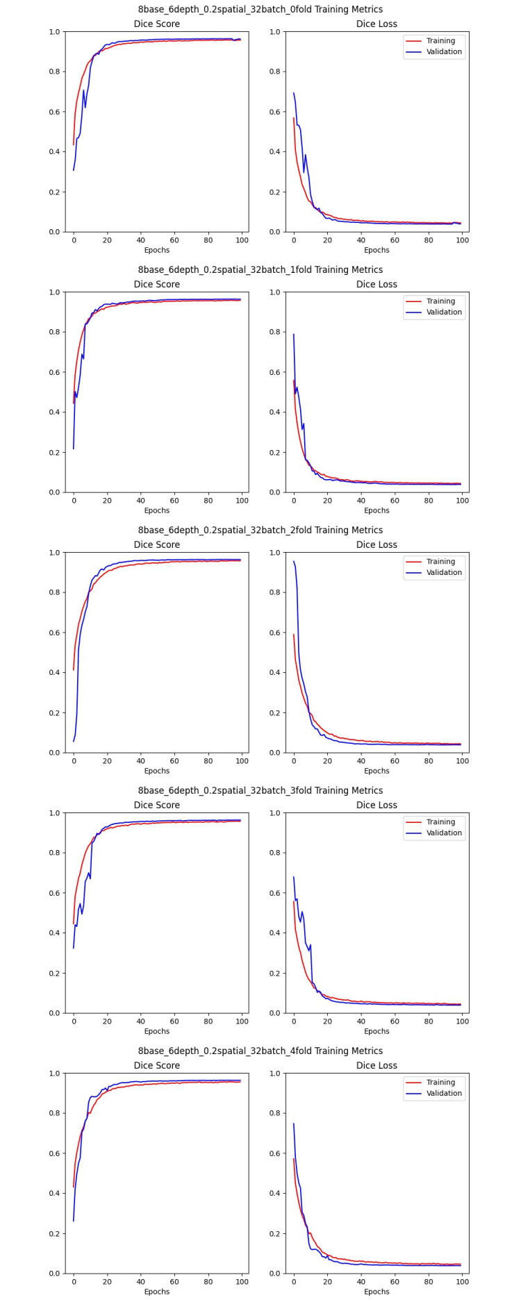
- Training graphs: These graphs should show how the accuracy and loss metrics develop from epoch to epoch for the training and validation set. They can help you determine if the model converges, when it begins to overfit, and the likelihood of data leakage.
- Statistics table: This table shows any relevant information for the model, such as the training set accuracy at the end of the last training epoch, the validation set accuracy, and the number of parameters in the model.
- Model Architecture: Information about the structure of the model itself. Tensorflow has a built-in function for visualizing this quickly.
- Visualized Inference: This portion of the report will look a lot like the input verification report for the validation set, but it will also include both the human and AI annotations. We place the worst performers at the top of the report to help focus analysis and subsequent iteration.
Model Comparison Report 🔗
During the development of any ML model, there are likely to be hundreds of models trained, each with different hyperparameters, data augmentations, or even different architecture configurations. Additionally, model improvements are likely to be made in the post-market phase as more data is acquired and newer ML techniques are discovered. Therefore, it is essential to have a way to compare multiple models so that you can empirically determine which model performs better. The model comparison report includes the training graphs for each of the models, a statistics table for easy model comparison, and the inferences from each of the models on the same validation dataset. Visualizing all of the different models’ inferences is particularly important since the loss function alone is not the full story. For example, a model with worse metrics could be because it is actually finding more human annotation errors than the others.
The Process 🔗
The process we have developed is rooted in the idea that good machine learning practices will lead to algorithms that will generalize to a real clinical setting and thus be safe and reliable. Here I’ll use an example project, segmenting the lungs in chest x-rays, to go step-by-step through our development process. I’ll be detailing the use of the four reports and pointing out common sources of errors along the way.
Step 1: Problem definition 🔗
When beginning any project, it is vital to understand the goals and limitations. We work closely with our clients to make sure that we can meet all their requirements. Some important considerations are:
- Speed: Should this run on an embedded device? Should inference be possible without a GPU? How many concurrent inferences are necessary and on what hardware?
- Accuracy: What accuracy do we think is necessary for a clinically useful model? If an algorithm suggests a segmentation for the physician to edit, the minimum accuracy threshold is probably lower than if the algorithm’s segmentations are used directly for diagnosis. A risk analysis coupled with a literature review can help determine this threshold.
- Development budget: Where should we be on the 80/20 rule? Each .9% added to the accuracy target will scale the cost exponentially. Should we use off the shelf architectures or something more customized? How fast do we need to develop the model? Is this a feasibility study, or do we need to observe more rigorous medical device design controls?
Example: For the Lung Segmentation problem, it doesn’t need to run on an embedded device and should always have access to a GPU. The goal is to make the model as accurate as possible, but there will usually be several inferences running concurrently. Ideally, the model will be as small as possible without sacrificing accuracy, as inferences time is related to model size. The budget and timeline are limited, so existing architecture implementations are preferred.
Step 2: Get data 🔗
The data used to train and test the model is an essential part of ML development. If a client already has a dataset ready to go, that’s great! But if not, we are happy to connect them with tools and services for image annotation as needed.
Example: I chose to go with a dataset from Kaggle, a machine learning hub where users can find and publish datasets and other resources to advance the data science field. Link to the dataset I used: https://www.kaggle.com/nikhilpandey360/chest-xray-masks-and-labels
Step 3: Data partition strategy 🔗
Once we have a dataset, there are several data processing steps to get it into a form readily consumable by ML. Usually, this involves splitting the dataset into training, validation, and test sets.
First, we work with our client to set aside a test set. The test set should be reasonably representative of the data commonly seen in clinical scenarios. It will not be used at all during model training. Instead, we will use it to see how well the algorithm performs on unseen data. It will also be the “acceptance criteria” used for the final deliverable and to verify the validity of incremental changes in future versions of the model.
After setting aside the test set, we split the remaining data into training and validation sets. It is common to use about twenty percent of the dataset for validation and the rest for training. Some errors to look out for are:
- Class imbalance: If you have several different classes, but one happens to end up exclusively in the validation set, the model will perform poorly on that class. To combat this, we try to ensure all of the classes are proportionally represented in each set. This technique is known as data stratification, and it is useful in many situations.
- Data leakage: This is the phenomenon that occurs when the validation set contains data that is too similar to the test set, so it is no longer a good indicator of how well the model performs on unseen data. Data leaks are especially common when the dataset contains clusters of very similar images. If those clusters are scattered among the training and validation sets, then it is as if the model has already ‘seen’ the validation set and will perform better than expected. Data leaks can mask overfitting, and solutions can vary depending on the data’s characteristics; Generally, you should keep related clusters together.
- Train/test ratio imbalance: How much data to set aside for validation? The validation set uses up data that could be used for training. A too-large validation set will result in a smaller training set, resulting in overfitting and decreased model performance. A too-small validation set will increase the likelihood of undetectable overfitting. Is it possible to make use of all your expensive annotation data while still detecting overfitting?
We highly recommend using the 5-fold cross-validation technique as it can help mitigate these problems. We split the data into five roughly equal ‘folds.’ Each fold should have data stratification and avoid data leakage. They should also be about the same ‘difficulty.’ When the folds are evenly split, we can use any one of the folds as the validation set during model training, and the remaining four form the training set. We can then combine the five models to produce a single model trained with all of the data. This technique has many advantages and few disadvantages beyond the setup time and complexity.
Example: After a careful look at the dataset, there don’t seem to be any clusters; each x-ray is of a different patient. But they are classified as either positive or negative for tuberculosis, and two hospitals took the scans. So I decided to simply split the data into six sets (five ‘folds’ and a test set) stratified by TB status and hospital of origin.
Step 4: Input verification reports 🔗
Before we start training any models, we need to be sure that all the work we’ve done on the dataset is successful! To this end, we generate an input verification report for each of the five folds and the test set, which will help us avoid another common error:
- Data Import Errors: Errors may occur when converting data to a format readily consumable by machine learning. For example, segmentation annotations may need to be transposed, or classification labels may have been improperly decoded. By visually inspecting the entire dataset before training, you can confirm the annotations and images the computer sees are what we expect, thereby de-risking the data loading process.
Example: As you can see in the sample below, I discovered some inconsistency in the segmentation annotations. Some include the heart, while others do not. I don’t have the budget to alter the segmentations, but I’ll have to keep this in mind when evaluating my models’ performance. On a client project, we would seriously consider reannotating the problematic data.
Step 5: Data augmentation 🔗
So I know it seems I’ve said all there is to say about the dataset, but we must take one last step before we start model training. Data augmentation can increase the effective size of your dataset and helps curb one of the most common ML errors:
- Overfitting: A phenomenon where a model simply ‘memorizes’ the training set. Overfitting can occur for a variety of reasons including insufficient data, overly complex model architecture, or training for too long. A symptom of this is a training accuracy that is much higher than the validation accuracy. Simultaneously, the validation set accuracy will decrease (unless you have data leakage). This is similar to how a student who merely memorizes the practice test will fail the real exam.
Data augmentation can take many forms, including but not limited to: zoom, rotate, mirror, and shift. While we highly recommend using data augmentation, it adds a new possible source of error:
- Over augmentation: When image augmentation is pushed to the limits, the original image can become unrecognizable or unrealistic. The range of realistic augmentations usually requires an expert opinion.
Data augmentation QA reports help us ensure that our data augmentation algorithm is effective and maintains our dataset’s integrity.
Example: Because chest x-rays vary naturally due to the machine’s exact placement in relation to the person, a certain amount of zoom and rotation makes sense. Similarly, some people are slightly taller or wider than others, so I allowed horizontal and vertical stretching. I disallowed horizontal flipping since this would unrealistically move the heart and other anatomy to the wrong side of the chest. Similarly, I disallowed vertical flipping since this scenario is easily corrected by looking at the DICOM tags as part of the pre-processing stage. For my report, I chose twelve random images from the dataset and generated ten augmented versions of each of them. After examining the first report, I realized that the rotation and stretch allowances were a bit too high, so I adjusted them appropriately. Below is an example from the final data augmentation QA report.
Step 6: Train a reference model 🔗
Now that our dataset is partitioned and augmented, we are ready to start training models. But whatever the model implementation we’ve chosen to use, there are still a lot of choices to make. How big of a model do we need? What are the best hyperparameters for our model? How many epochs should we train? Maybe we even have several architectures to choose from. Whatever the case, we like to start with some ‘reasonable’ parameters and do a full round of 5-fold cross-validation training. The resulting five models will be identical except for which of the folds is the validation set, and we’ll generate a model performance report for each of them. We do this for a few reasons:
- Fold imbalance: While we try to make all of our folds equal, it is hard to know if we’ve succeeded until we’ve used each of them as the validation set. By comparing the training graphs and statistics tables in the model performance reports, we can see if any of the folds are more or less ‘difficult’ than the others and make corrections as necessary.
- Overfitting: By comparing the training graphs, we can see when each of the models begins to converge. While this will differ depending on the architecture, it can give you a reasonable idea of how long to train the models during your hyperparameter searches.
- Unreasonable parameters: If the reference model doesn’t converge, the model may be too simple. This phenomenon is also called underfitting. If it converges and begins to overfit very quickly, the model could be too complex. Sometimes you get lucky, and the model performs well, so you know you are at least in the ballpark. Whatever the case, these models’ performance can help you choose reasonable ranges for a hyperparameter search.
- Bad accuracy metric: Different problems have different ways of measuring accuracy. For a binary classification problem, accuracy could be just whether or not the model guessed correctly. For image segmentation, we usually use the Dice similarity score. But if the metric you use doesn’t suit your problem, the training graphs and statistics will look like the model performs poorly. Visualizing the inferences on the validation set will also give you a good idea of whether your accuracy metric is calculated correctly and correlates with clinical objectives.
- Architecture selection: If you have a choice of several model implementations, repeating this exercise with each architecture will hopefully help you narrow down your options.
Example: I chose a U-net implementation that is commonly used for medical imaging segmentation tasks. I also used hyperparameters that I knew worked well for previous projects. I got lucky. They all begin to converge at about 20 epochs, and the validation set Dice scores were all 95 - 96%, so the folds are balanced. I trained for 100 epochs, and it only just began to overfit, if at all, so I’ll probably stick with that for my hyperparameter search. Here are the training graphs for the five models:
Step 7: Broad hyperparameter search 🔗
A hyperparameter is a training variable that can influence the resulting model’s performance. Many model architectures will have default hyperparameter values that work ‘pretty well’ in most cases. Still, every problem will have a unique combination of hyperparameter values that will produce the best model. This is because each problem has a unique “difficulty level” that is difficult to gauge prior to the hyperparameter search. More difficult problems requires a more complex model while simpler problems should only need a simple model. A hyperparameter search trains many different models to find the ideal combination of variables. As a general rule, it is best to pick the simplest model possible that achieves your clinical objectives since simpler models are less likely to overfit.
It is good to choose a wide range of values for each of the hyperparameters to get enough models to be useful. We also select one of the folds to be the validation set for each of the models because it reduces training time (only one model per hyperparameter combination). When making model comparison reports, the models all must have the same validation set anyway.
The method of the search can vary as well. Randomly checking various parameter combinations is common, and optimization algorithms can help narrow down the search. We usually end up with many models, each with a model performance report, whatever technique we use. Now the question becomes, how do we choose the best one?
Example: The U-net architecture I chose has three main hyperparameters: the number of filters at the first convolutional layer (base size), the number of convolutional layers (depth), and the spatial dropout fraction. I also varied the batch size, which gave me a total of four hyperparameters. I chose to do a random search, and I ended up with 200 models after letting it train overnight on 4 GPUs.
Step 8: Model comparison reports 🔗
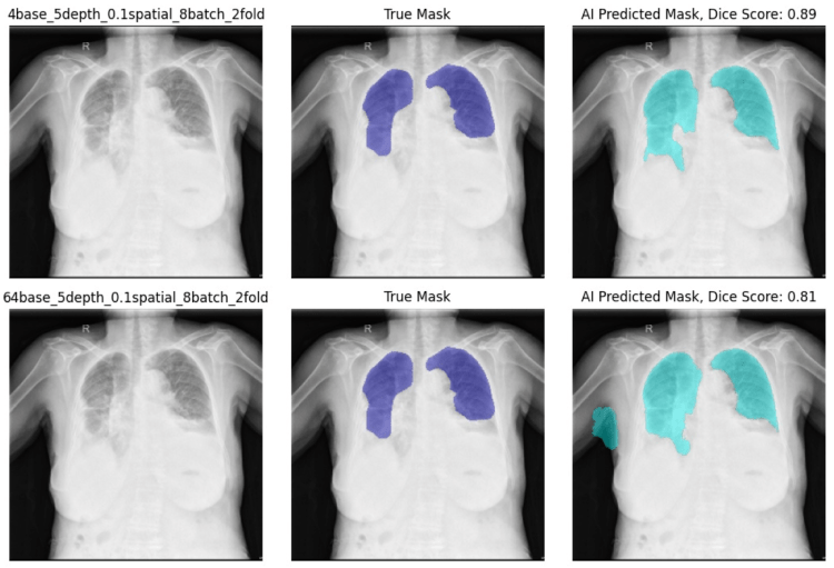
Model comparison reports allow us to efficiently compare many models to find patterns in the results that will point us toward the ideal hyperparameter combination. We generally try to compare models that are identical in every way except for one hyperparameter to give some context; how does that particular variable influence the model? This step’s primary goal is to narrow down the range of hyperparameter values for the next step. Secondarily, the hyperparameter search also allows us the opportunity to gain more confidence in the architecture and methods by demonstrating hyperparameters tweaks are having the expected result on the output.
Example: I created four model comparison reports, one for each hyperparameter. Almost every model I looked at had a validation set accuracy of 95% or 96%, no matter how complex. Qualitatively, all models were performing comparably even with the more difficult images that all of them struggled with. The “deep” models (more convolutional layers) performed better, and the models with a spatial drop-out rate of 0.2 performed worse than 0.0 or 0.1. I also noted that the training batch size made a difference. The larger batch sizes took longer to converge and performed more poorly in general.
| Model Name | Training Dice Score | Validation Dice Score | Total Parameters |
|---|---|---|---|
| 8base_3depth_0.2spatial_32batch_2fold | 0.95 | 0.96 | 123,533 |
| 8base_4depth_0.2spatial_32batch_2fold | 0.95 | 0.96 | 494,093 |
| 8base_5depth_0.2spatial_32batch_2fold | 0.96 | 0.96 | 1,972,493 |
| 8base_6depth_0.2spatial_32batch_2fold | 0.96 | 0.96 | 7,878,413 |
| 8base_7depth_0.2spatial_32batch_2fold | 0.96 | 0.96 | 31,486,733 |
Additionally, the larger filter base size models performed worse than the smaller ones, though the difference was more subtle. As you can see in the report below, the model with a filter base size of 64 marked some of the right arm as lung, while the model with a filter base size of 4 did not.
Step 9: Narrow hyperparameter search 🔗
After examining the model comparison reports, we usually have a good idea of how the various hyperparameters affect the model performance. We can then adjust the hyperparameter ranges to perform a more targeted or expanded search. Once the training is complete, we use model comparison reports to find the best models and continue to iterate if necessary.
Example: I reduced the filter base size range, reduced the batch size range, and shifted the layer depths upwards. I ended up with 74 models, and they all had great dice scores. After making several model comparison reports and reviewing them closely, I ended up with two models that performed similarly.
Step 10: 5-Fold cross-validation 🔗
Now that we have narrowed down the list to just one model (if we’re lucky), or maybe the top three, it is time to run the full 5-fold cross validation training on each of the finalists. The goal is to get enough information to choose your model parameters and determine exactly how many epochs you need to train to converge without overfitting.
Example: I ran 5-fold cross-validation training on the two best models. I reduced my training time to 50 epochs as all of the models in the hyperparameter searches had converged by that point and I wanted to make sure I wasn’t overfitting. I chose the second model to continue because the first model had a consistently lower training dice score than the second.
Step 11: Whole dataset training 🔗
At this point, we want to celebrate, but there is a bit more work to be done. We have the right combination of hyperparameters, we know how long to train the model, and we have five great models —one for each fold— that all do a good job of segmenting our images. But to make the best use of our dataset, we want to use as much data as possible in the training set. In order to do this, we use all five folds for training (with no validation set). Usually, the danger in having no validation set is that you have no way to know if you are overfitting or not. But because of the previous 5-fold cross-validation experiments, we know exactly how long we can train without overfitting.
Example: Once I finished training my model on all five folds, I got 96% accuracy on the test set. Ultimately all of the models throughout the process struggled because the segmentations were inconsistent. In every fold, the images that always had the lowest Dice score were the ones that had the heart included in the annotation. This shows how important it is to have a consistent dataset. Ideally, I would have taken the time to edit the annotations myself, but for this article, I think it is good to show that no amount of data augmentation or training will make up for bad data.
Step 12: Model acceptance 🔗
The final step in the model development process is to see how it performs on the test set that was set aside at the very beginning. We create a final model performance report with the test set as the validation set. Assuming the accuracy metrics meet the acceptance criteria, we’re done!
Well, not done-done. The model still needs to be incorporated into the product, and it will need updates as more data is collected. But with the reports produced throughout this model development process, you’ll be ready to navigate the FDA approval/clearance process.
Step 13: Maintenance and post-market surveillance 🔗
Once your model is deployed you will likely want to make changes as more data and ML techniques are available. The same techniques we discussed in this article apply to both adaptive and non-adaptive algorithms. The model comparison report, in particular, is well suited to compare version 2.0 of the algorithm to version 1.0 that was cleared by the FDA.
Step 14: Book a consultation 🔗
You made it to the end! If you got this far and would us to help you take your algorithm to the next step, please book a consultation today!
Acknowledgments 🔗
1 Special thanks to Nick Schmansky, CEO of Corticometrics for pointing out these additional pitfalls.