Medical imaging isn’t easy for computer vision engineers—coordinate systems, image orientations, and subtle data-quality issues cause otherwise strong AI models to fail validation. Even experienced ML engineers trip over common but avoidable mistakes like incorrectly flipping images, mixing anatomical directions, or misaligning voxel coordinates. This guide is for engineers moving into medical imaging who want practical, direct advice on what to do (and what not to do).
Inside, you’ll find clear examples and best practices to:
- Normalize images consistently to canonical coordinates (RAS/LPS)
- Check and correct anatomical orientations upfront
- Validate reconstruction kernels early to avoid domain shift surprises
- Properly handle indexing and augmentation to maintain anatomical accuracy
My goal is to give you simple checks and actionable insights—without unnecessary theory—to quickly avoid the pitfalls that stall projects and delay FDA submissions. For regulatory context, you might also read my articles on FDA submission strategies for general AI models, using command-line interfaces for faster clearances, and converting user needs into clear engineering requirements.
Follow these guidelines to ship medical-imaging AI models that work reliably, pass validation the first time, and let you move faster on what matters most: building better products.
Handling Core Image Encoding Issues 🔗
-
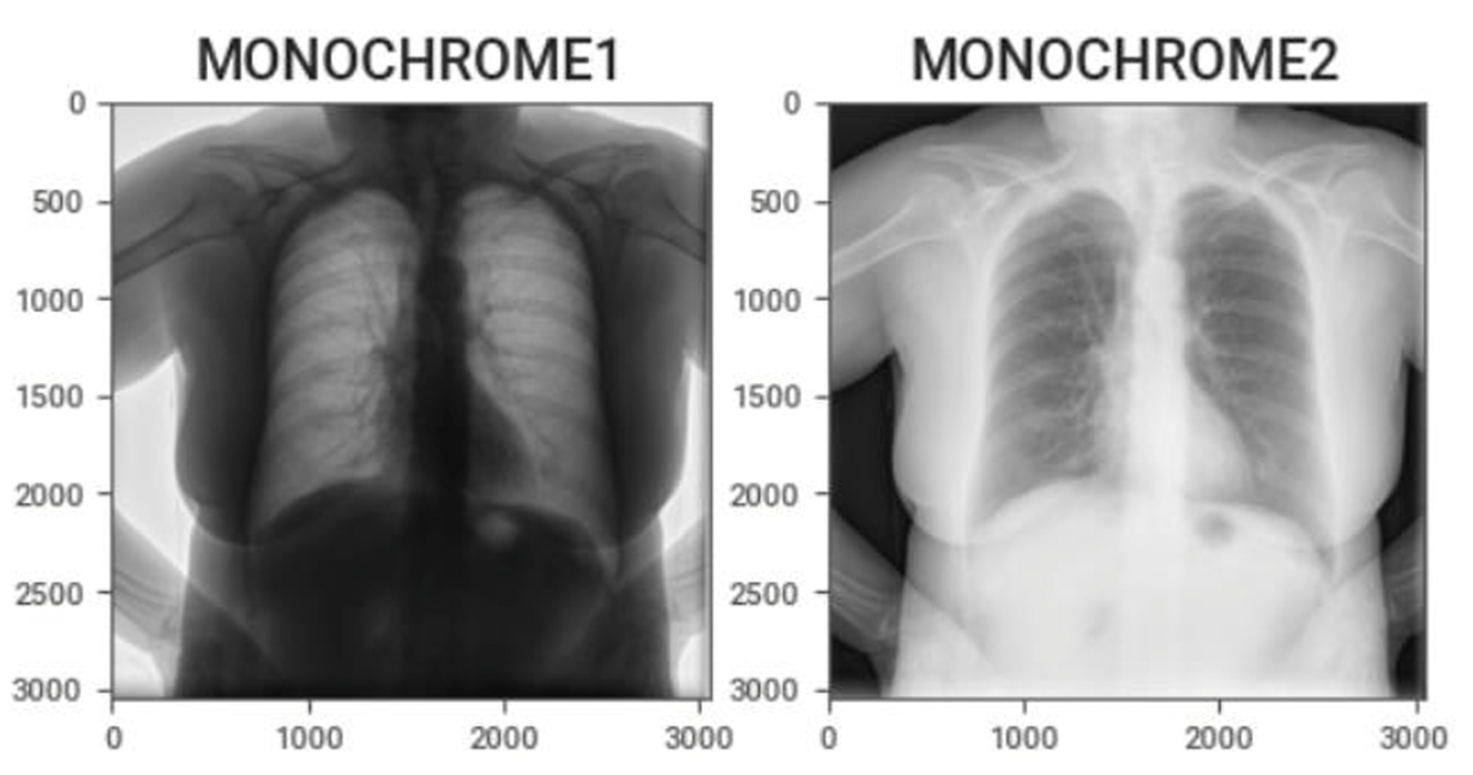
Omitting photometric inversion for MONOCHROME1 images Basic:
The DICOM attribute Photometric Interpretation (0028,0004) specifies the intended interpretation of the pixel data
- MONOCHROME1 : The minimum sample value is intended to be displayed as white. Higher pixel values represent darker shades, and lower pixel values represent brighter shades.
- MONOCHROME2 : The minimum sample value is intended to be displayed as black. Higher pixel values represent brighter shades, and lower pixel values represent darker shades.
Problem:
If MONOCHROME1 images are not corrected through photometric inversion, the structures like bones, air, or soft tissue appear visually reversed, which can confuse machine learning models. If MONOCHROME1 images are used without correction, models may learn incorrect intensity features, resulting in poor generalization and reduced accuracy. Furthermore, keeping MONOCHROME1 images in the same dataset with MONOCHROME2 images leads to inconsistency, non-reproducible results, and may lead to processing errors in tasks like thresholding or segmentation. Correcting MONOCHROME1 images is essential for maintaining consistency and ensuring reliable model training.
Recommended Approach:
- Detect Photometric Interpretation.
- If MONOCHROME1, invert the image values (but don’t invert padding).
- Normalize intensities consistently across all inputs before feeding into ML.
Example:
Sample code:
from pydicom import dcmread from pydicom.uid import generate_uid import numpy as np def invert_mono1_to_mono2(in_file, out_file): ds = dcmread(in_file) if ds.PhotometricInterpretation != "MONOCHROME1": print("No inversion needed.") return arr = ds.pixel_array.astype(np.int32) # Handle padding value if present pad_val = getattr(ds, "PixelPaddingValue", None) mask = (arr == pad_val) if pad_val is not None else None # Check pixel representation: 0 = unsigned, 1 = signed if ds.PixelRepresentation == 0: max_val = (1 << ds.BitsStored) - 1 arr = max_val - arr else: min_val = -(1 << (ds.BitsStored - 1)) max_val = (1 << (ds.BitsStored - 1)) - 1 arr = max_val - (arr - min_val) # Restore padding if mask is not None: arr[mask] = pad_val # Update dataset ds.PixelData = arr.astype(ds.pixel_array.dtype).tobytes() ds.PhotometricInterpretation = "MONOCHROME2" # Generate new UID new_uid = generate_uid() ds.SOPInstanceUID = new_uid ds.file_meta.MediaStorageSOPInstanceUID = new_uid # Save file ds.save_as(out_file, write_like_original=False) print(f"Converted and saved: {out_file}") # Example usage invert_mono1_to_mono2("input.dcm", "output.dcm") -
HU calibration (CT) often ignored or inconsistently applied Basic:
The Hounsfield scale is a quantitative scale for describing radiodensity in medical CT and provides an accurate density for the type of tissue. On the Hounsfield scale, air is represented by a value of −1000 (black on the grey scale) and bone between +700 (cancellous bone) to +3000 (dense bone) (white on the grey scale). In CT imaging, the raw pixel values stored in DICOM files are not always directly Hounsfield Units (HU).
Rescale intercept, (0028, 1052), and rescale slope (0028, 1053) are DICOM tags that specify the linear transformation from pixels in their stored on disk representation to their in memory
U = m*SV + b
where U is in output units, m is the rescale slope, SV is the stored value, and b is the rescale intercept.
Problem:
- Some scanners or PACS export CT slices already in HU, while others store uncalibrated pixel values with slope/intercept metadata.
- If this calibration is skipped, identical tissues appear at different intensity levels across datasets. This creates artificial domain shifts, leading AI models to misinterpret and struggle with generalization.
Recommended approach:
Apply the rescale slope and intercept to all CT images to convert raw pixel values into Hounsfield Units (HU), unless the images are already stored in HU.
Sample code:
from pydicom import dcmread import numpy as np def get_hu_image(dcm_file): ds = dcmread(dcm_file) arr = ds.pixel_array.astype(np.int16) slope = float(getattr(ds, "RescaleSlope", 1.0)) intercept = float(getattr(ds, "RescaleIntercept", 0.0)) # Apply calibration hu_img = arr * slope + intercept # Optional: clip to standard HU range hu_img = np.clip(hu_img, -1000, 3000) return hu_img # Example hu_image = get_hu_image("ct_slice.dcm") print("HU range:", hu_image.min(), "to", hu_image.max()) -
Incorrect handling of signed vs unsigned pixel values → mis-scaled images Basic:
Encoded pixel data of various bit depths must be correctly interpreted. These DICOM elements define the pixel structure:
- Bits Allocated (0028,0100): Number of bits used for each pixel sample (e.g., 16).
- Bits Stored (0028,0101): Number of meaningful bits that actually encode pixel intensity (e.g., 12).
- High Bit (0028,0102): The position of the most significant bit in the stored pixel sample.
- Pixel Representation (0028,0103): Defines whether the stored values are unsigned (0) or signed (1).
Problem:
- Misinterpreting signed vs unsigned values (Pixel Representation) causes negative Hounsfield Units to be incorrectly read as large positive values. For example a voxel with HU = −1000 may appear as 64536 if interpreted as unsigned 16-bit. For AI/ML pipelines, this leads to inconsistent intensity scaling, artificial domain shifts, and unreliable training data.
- Ignoring the High Bit can shift pixel ranges, creating intensity values that do not match reality.
Recommended Approach:
- Read all relevant attributes (BitsAllocated, BitsStored, HighBit, PixelRepresentation).
- Align and mask the stored values:
- Right-shift so that the meaningful bits start at bit 0.
- Mask with (1 << BitsStored) - 1.
- Apply sign conversion if PixelRepresentation == 1 (signed).
- Preserve padding values (don’t apply rescale to them).
Sample code:
import numpy as np
import pydicom

def decode_pixels(ds):
    raw = ds.pixel_array.astype(np.uint16)

    bits_alloc = int(ds.BitsAllocated)
    bits_stored = int(ds.BitsStored)
    high_bit = int(ds.HighBit)
    pix_repr = int(ds.PixelRepresentation)  # 0=unsigned, 1=signed

    # Align meaningful bits
    shift = high_bit - (bits_stored - 1)
    vals = raw >> shift if shift >= 0 else raw << (-shift)

    mask = (1 << bits_stored) - 1
    vals = vals & mask

    # Apply sign if needed
    if pix_repr == 1:
        sign_bit = 1 << (bits_stored - 1)
        vals = vals.astype(np.int32)
        vals[vals & sign_bit != 0] -= (1 << bits_stored)

    # Apply rescale (if present)
    slope = float(getattr(ds, "RescaleSlope", 1.0))
    intercept = float(getattr(ds, "RescaleIntercept", 0.0))
    vals = vals * slope + intercept

    return vals.astype(np.float32)
Acquisition and Series-Level Gotchas 🔗
-
Multiple series per study naively combined into one dataset Basic:
A Series is a group of images that share the same acquisition and reconstruction parameters. Multiple series refers to a collection of distinct sets of images or data acquired during a single medical imaging study.
A single DICOM study may contain multiple series:
- Different acquisition phases (time points, breath-hold, systole vs diastole).
- Different reconstruction settings (kernel, slice thickness, field of view).
- Different orientations or modalities (axial, MPR, localizer).
If these series are naively combined into one dataset, AI/ML models may learn inconsistent image textures, intensity distributions, and anatomical states.
Problem:
- Mixing reconstructions: Sharp kernels exaggerate edges/noise, while smooth kernels blur details. Combining them confuses models trained for detection/quantification.
- Mixing temporal phases: A lesion or vessel may look different in systole vs diastole. Without labeling, the model sees this as contradictory data.
- Slice thickness / orientation mismatches: Can cause voxel size inconsistencies, breaking 3D CNNs or volumetric analysis.
Recommended Approach:
- Group images by SeriesInstanceUID to separate image sets.
- Extract series-level attributes such as SeriesDescription, ConvolutionKernel, SliceThickness, PixelSpacing, ImageOrientationPatient, TemporalPositionIdentifier, and TriggerTime.
- Decide which series to keep depending on the task. For example, for coronary plaque or FFR analysis, prefer diastolic phase and smooth kernel.
- Validate consistency within each selected series, ensuring the same kernel, slice thickness, pixel spacing, and orientation. If inconsistencies are found, exclude or resample that series.
Sample Code:
import os from collections import defaultdict import pydicom def group_by_series(dicom_dir): series_dict = defaultdict(list) for fname in os.listdir(dicom_dir): if not fname.endswith(".dcm"): continue ds = pydicom.dcmread(os.path.join(dicom_dir, fname), stop_before_pixels=True) series_uid = ds.SeriesInstanceUID desc = getattr(ds, "SeriesDescription", "Unknown") kernel = getattr(ds, "ConvolutionKernel", "Unknown") series_dict[(series_uid, desc, kernel)].append(fname) return series_dict # Example usage dicom_dir = "study_folder/" series_info = group_by_series(dicom_dir) for (uid, desc, kernel), files in series_info.items(): print(f"Series: {uid}") print(f" Description: {desc}") print(f" Kernel: {kernel}") print(f" Num images: {len(files)}\n") -
Non-sequential Acquisition Number & Instance Number ordering Basic:
Acquisition Number (0020,0012) is a number identifying the single continuous gathering of data over a period of time that resulted in this instance. The Instance Number is a numerical value found in the (0020,0013) attribute that identifies a specific image or instance within a series.
Problem:
In DICOM series, AcquisitionNumber and InstanceNumber may not be sequential or consistent across slices. This non-sequential numbering can lead to incorrect slice ordering, misaligned stacks, or volume misreconstruction during 3D reconstruction.
Recommended Approach:
Do not rely solely on AcquisitionNumber or InstanceNumber for ordering. Instead, group by AcquisitionNumber (or SeriesInstanceUID if multiple series exist) and sort images using spatial information: ImagePositionPatient (0020,0032) for slice location and ImageOrientationPatient (0020,0037) for orientation.
Sample Code:
import pydicom import glob # Load DICOM files files = [pydicom.dcmread(f) for f in glob.glob("path/to/dicom/*.dcm")] # Sort by spatial location (z-coordinate in ImagePositionPatient) slices = sorted(files, key=lambda d: float(d.ImagePositionPatient[2])) # Reconstructed volume stack volume = [s.pixel_array for s in slices] -
Multi-frame vs Single-frame DICOMs Basic:
A single-frame DICOM stores one image (frame) per file, common in CT and MR series. A multi-frame DICOM stores an entire temporal or spatial sequence (e.g., ultrasound cine loops, MR perfusion, functional imaging) within a single file using the (0028,0008) Number of Frames attribute.
Problem:
Handling multi-frame and single-frame DICOMs uniformly can be challenging. Multi-frame files bundle all frames in one instance, while single-frame series store each frame separately across multiple files. This difference can cause parsing issues, inconsistent data handling, or missing time-series information if not properly accounted for.
Recommended Approach:
- Check for (0028,0008) Number of Frames to detect multi-frame images.
- For multi-frame, extract frames directly from the single file.
- For single-frame, collect and sort all instances (using InstanceNumber or ImagePositionPatient) before stacking.
Sample Code:
import pydicom
import numpy as np
import glob

# Read one DICOM file
ds = pydicom.dcmread("example.dcm")

if hasattr(ds, "NumberOfFrames"):
    # Multi-frame DICOM
    frames = ds.pixel_array  # Shape: (num_frames, rows, cols)
else:
    # Single-frame DICOM series
    files = [pydicom.dcmread(f) for f in glob.glob("series/*.dcm")]
    files = sorted(files, key=lambda d: int(d.InstanceNumber))
    frames = np.stack([f.pixel_array for f in files])  # Shape: (num_frames, rows, cols)

print("Frames shape:", frames.shape)
Checking the Reconstruction Kernel 🔗
Basic:
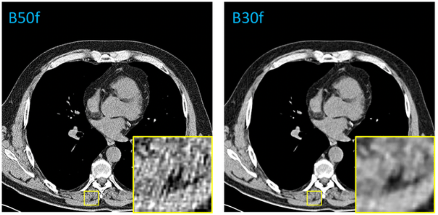
The kernel, often referring to a convolution kernel, refers to the process used to modify the frequency contents of projection data prior to back projection during image reconstruction in a CT scanner. The selection of reconstruction kernel should be based on specific clinical applications. There is a tradeoff between spatial resolution and noise for each kernel. A smoother kernel generates images with lower noise but with reduced spatial resolution. A sharper kernel generates images with higher spatial resolution, but increases the image noise. For example, smooth kernels are usually used in brain exams or liver tumor assessment to reduce image noise and enhance low contrast detectability, whereas sharper kernels are usually used in exams to assess bony structures due to the clinical requirement of better spatial resolution.
Problem:
- Reconstruction kernels significantly alter image characteristics such as sharpness, noise, and texture. This directly impacts how anatomical structures appear in CT images, which can mislead AI models if not standardized.
- AI models are sensitive to variations in input data, and differences in kernels create a domain shift between training and inference data. If a model is trained on soft kernels but tested on sharp ones, its performance can drop due to mismatched textures and edge clarity.
- Vendor-specific naming and implementation of kernels add complexity, making it essential to normalize or filter datasets based on kernel type to ensure consistency across studies or institutions.
- Ignoring reconstruction kernels can lead to degraded model performance, bias, and poor generalizability.
Recommended Approach:
- Extract the reconstruction kernel information from the DICOM metadata using the tag
0018,1210. This value indicates the type of convolution kernel applied during image reconstruction and must be reviewed before using the scan for model training or inference. - Normalize the kernel names to account for variations across scanner vendors.
- Incorporate kernel checking as a preprocessing step before any model development or analysis. This ensures that kernel-based variability does not silently affect the model’s performance, particularly in sensitive tasks like segmentation, radiomics, or classification.
- Apply harmonization techniques if dataset include scans with different kernels. This could involve using smoothing filters, histogram matching, radiomic feature normalization (e.g., ComBat), or advanced domain adaptation strategies to minimize the impact of kernel differences on model generalization.
Example:
Reconstruction kernels used on lungs CT
Hard Kernel Soft Kernel
Sample Code:
import pydicom
# Check reconstruction kernel from a DICOM file
def check_kernel(dicom_path, accepted_kernels={"SOFT_TISSUE"}):
    try:
        ds = pydicom.dcmread(dicom_path, stop_before_pixels=True)
        kernel = ds.get("ReconstructionKernel", "").strip()
        if not kernel:
            print(f"{dicom_path}: No kernel info found.")
            return None
        category = normalize_kernel(kernel)
        print(f"{os.path.basename(dicom_path)} | Kernel: {kernel} | Category: {category}")
        if category in accepted_kernels:
            return "Accepted"
        else:
            return "Rejected"
    except Exception as e:
        print(f" Error processing {dicom_path}: {e}")
        return None
import os
import numpy as np
import SimpleITK as sitk
from skimage.exposure import match_histograms
import pandas as pd
from neuroHarmonize import harmonizationLearn, harmonizationApply

# Apply Smoothing to Sharp Kernels
def apply_smoothing(image, sigma=1.0):
    """Apply Gaussian smoothing to reduce edge artifacts from sharp kernels."""
    return sitk.DiscreteGaussian(image, sigma)

# Histogram Matching to Reference Scan
def match_histogram_to_reference(moving_image, reference_image):
    """Match histogram of moving_image to reference_image using scikit-image."""
    moving_np = sitk.GetArrayFromImage(moving_image)
    ref_np = sitk.GetArrayFromImage(reference_image)
    matched = match_histograms(moving_np, ref_np, multichannel=False)
    return sitk.GetImageFromArray(matched.astype(moving_np.dtype))

# Radiomics Feature Harmonization with ComBat
def harmonize_features_combat(features_df, batch_labels):
    """
    Apply ComBat harmonization to radiomics features.
    features_df: DataFrame with rows=samples, cols=features
    batch_labels: List or array with batch (kernel) labels
    """
    model, data_transformed = harmonizationLearn(features_df.values, batch_labels)
    df_harmonized = pd.DataFrame(data_transformed, columns=features_df.columns)
    return df_harmonized
Hanging Protocol and Display Quirks 🔗
-
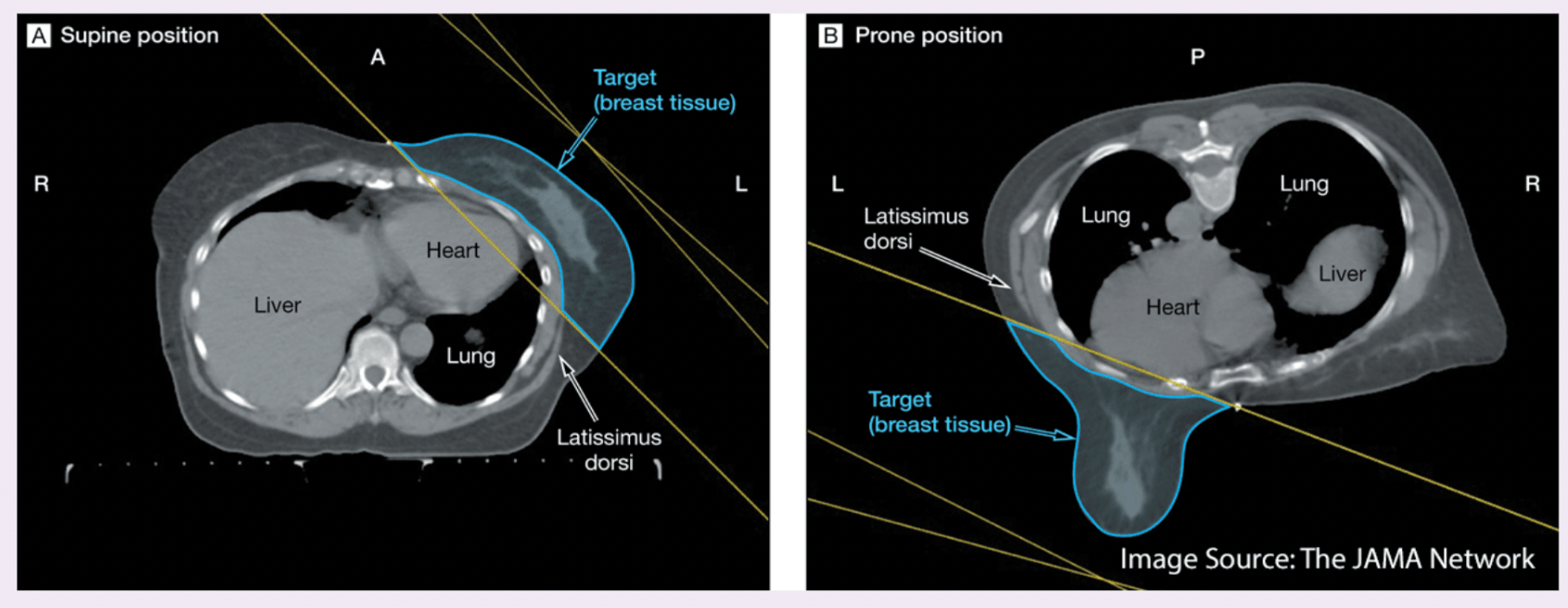
Reconcile prone/supine orientation before label propagation Basic:
CT and MRI scans can be acquired with the patient in different positions, most commonly supine (lying face up) or prone (lying face down). While the internal anatomy remains unchanged, the orientation in the image space differs, which can affect how labels align.
Problem:
Prone and supine scans of the same patient can differ dramatically in spatial orientation, even if taken on the same day. Without reconciling this difference, label propagation (transferring segmentation masks or contours from one scan to another) or training AI models across such scans can lead to severe spatial inconsistencies.
Key challenges include:
-
Orientation & Label Consistency Medical images encode orientation using metadata (e.g., DICOM Patient Position or Image Orientation tags like “Head First Prone” vs. “Head First Supine”). If this information is incorrect or ignored, scans may be flipped or rotated by 180°, misaligning anatomical structures.
Crucially, this affects label consistency. Segmentation masks or contours must align anatomically. Misinterpreting orientation can lead to mirrored, misplaced, or anatomically invalid labels, compromising both AI model training and evaluation.
-
Anatomical Deformation: Postural changes cause anatomical deformation. For instance:
- Organs may shift under gravity in prone vs. supine (e.g., in breast or abdominal imaging).
- The colon might distend or collapse differently in CT colonography. Even after correcting for orientation, such deformations may require deformable registration to align corresponding structures.
Recommended approach:
- Normalize to a Standard Orientation (e.g., LPS or RAS): Use libraries like SimpleITK to convert all scans to a consistent anatomical orientation using the direction cosines stored in the image headers.
- Perform Rigid or Deformable Registration (optional): After orientation normalization, apply rigid registration to account for translations and rotations. In cases where anatomy has shifted (e.g., due to posture or gravity), apply deformable registration to align internal structures more precisely. This depends upon the application and is not always required.
- Propagate Labels Using the Composite Transform: Once images are aligned, propagate segmentation labels using nearest-neighbor interpolation to preserve label integrity.
Example: CT images for breast cancer radiation
The left image shows the patient in the supine position (lying face up), while the right image shows the prone position (lying face down).
Sample Code:
import SimpleITK as sitk def normalize_orientation(image, orientation='LPS'): """Convert image to a standard anatomical orientation.""" return sitk.DICOMOrient(image, orientation) def rigid_register(fixed, moving): """Perform rigid registration using mutual information.""" initial_transform = sitk.CenteredTransformInitializer( fixed, moving, sitk.Euler3DTransform(), sitk.CenteredTransformInitializerFilter.GEOMETRY ) registration = sitk.ImageRegistrationMethod() registration.SetMetricAsMattesMutualInformation(50) registration.SetOptimizerAsRegularStepGradientDescent( learningRate=1.0, minStep=1e-4, numberOfIterations=100 ) registration.SetInterpolator(sitk.sitkLinear) registration.SetInitialTransform(initial_transform, inPlace=False) final_transform = registration.Execute(fixed, moving) return final_transform def deformable_register(fixed, moving, initial_transform=None): """Perform deformable B-spline registration.""" tx = sitk.BSplineTransformInitializer(fixed, [8, 8, 8]) registration = sitk.ImageRegistrationMethod() registration.SetInitialTransformAsBSpline(tx, inPlace=True, scaleFactors=[1, 2, 5]) registration.SetMetricAsMattesMutualInformation(50) registration.SetOptimizerAsGradientDescent(1.0, 100) registration.SetInterpolator(sitk.sitkLinear) transform = registration.Execute(fixed, moving) return transform def propagate_label(label_image, reference_image, transform): """Warp label image using nearest-neighbor interpolation.""" return sitk.Resample( label_image, reference_image, transform, sitk.sitkNearestNeighbor, 0, label_image.GetPixelID() ) -
-
CC vs MLO confusion in mammography Basic:
In each mammogram examination, a breast is typically imaged with two different views, i.e., the mediolateral oblique (MLO) view and cranial caudal (CC) view. The MLO view provides a side view, visualizing the greatest amount of breast tissue, including the posterior and axillary regions. The CC view offers a top-down perspective, showing deep medial breast tissue often excluded in the MLO view. These orientations provide complementary information and are essential for accurate diagnosis, follow-up studies, and AI-based analysis pipelines. In mammography, the View Position (0018, 5101) and Laterality (0020, 0060) DICOM tags play a crucial role in ensuring that images are correctly identified and interpreted.
Problem:
A common issue arises when view positions are mislabeled in the DICOM metadata. For example, a CC image may mistakenly be tagged as MLO or vice versa. This mislabeling disrupts automated pipelines that assume correct metadata, potentially leading to errors in image registration, training datasets for machine learning, and even clinical interpretations. Furthermore, if both views of the same breast are incorrectly labeled as CC or MLO, the completeness of the exam is compromised, which is especially critical in longitudinal breast cancer screening studies.
Recommended Approach:
- Check DICOM tags (View Position (0018, 5101) and Laterality (0020, 0060)) to confirm that both CC and MLO views are present for each breast.
- Cross-validate labels with pixel-level geometry or anatomical landmarks, such as the presence of the pectoral muscle (commonly seen only in MLO views).
Example:
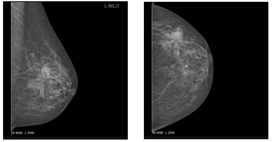
MLO CC
Sample Code:
import os import pydicom def check_mammo_view_positions(folder): results = [] for f in os.listdir(folder): if not f.endswith(".dcm"): continue ds = pydicom.dcmread(os.path.join(folder, f)) view = ds.get((0x0018, 0x5101), "Unknown") # View Position laterality = ds.get((0x0020, 0x0060), "Unknown") # Laterality fname = os.path.basename(f) results.append((fname, laterality, view)) print("=== Mammography View Position Check ===") for fname, lat, view in results: print(f"{fname}: Laterality={lat}, View={view}") # Quick consistency check views = [v for _, _, v in results if v != "Unknown"] if len(set(views)) < 2: print(" Potential issue: Missing either CC or MLO views.") else: print(" Both CC and MLO views detected.") # Example usage # check_mammo_view_positions("path/to/mammo/folder") -
Windowing metadata absent or vendor-specific Basic:
CT image values correspond to Hounsfield units (HU). But the values stored in CT Dicoms are not Hounsfield units, but instead a scaled version. To extract the Hounsfield units we need to apply a linear transformation, which can be deduced from the Dicom tags.
Once we have transformed the pixel values to Hounsfield units, we can apply a windowing. Windowing in medical imaging refers to the process of mapping raw pixel intensities (stored in Hounsfield units for CT or arbitrary vendor values for modalities like MR) into grayscale display values. This mapping is controlled by DICOM tags such as Window Center (0028, 1050) and Window Width (0028, 1051) , which define how intensities are rescaled for optimal visualization.
Problem:
If windowing metadata is absent or implemented in vendor-specific ways, the same image may appear differently depending on the viewing system. For AI pipelines, missing or inconsistent windowing tags may result in models being trained on differently scaled inputs, reducing reproducibility and cross-institutional generalizability.
Recommended Approach:
- Verify the presence of Window Center (0028, 1050) and Window Width (0028, 1051) in every image header.
- If missing, compute default values directly from pixel intensity distributions (e.g., mean/standard deviation or min/max).
- Standardize windowing in preprocessing by applying consistent intensity normalization across datasets (e.g., rescaling HU to [-1000, 400] for lung CT).
Sample Code:
import pydicom
import numpy as np
import matplotlib.pyplot as plt

def apply_windowing(ds):
    # Extract pixel array
    img = ds.pixel_array.astype(np.float32)

    # Try reading Window Center & Width
    try:
        center = float(ds.WindowCenter)
        width = float(ds.WindowWidth)
    except AttributeError:
        # If missing, compute default window from pixel range
        center = np.mean(img)
        width = np.max(img) - np.min(img)
        print(f"[INFO] Windowing tags missing, using computed defaults: Center={center}, Width={width}")

    # Apply windowing transformation
    lower = center - width / 2
    upper = center + width / 2
    img_windowed = np.clip(img, lower, upper)

    # Normalize to [0,255] for visualization or AI preprocessing
    img_norm = (img_windowed - lower) / (upper - lower)
    img_norm = (img_norm * 255).astype(np.uint8)

    return img_norm

# Example usage
dcm_path = "example_ct.dcm"  # replace with your CT DICOM file
ds = pydicom.dcmread(dcm_path)
processed_img = apply_windowing(ds)

# Show processed image
plt.imshow(processed_img, cmap="gray")
plt.title("Windowed & Normalized CT")
plt.axis("off")
plt.show()
Patient & Metadata Confounders 🔗
-
Confusion between Pixel Spacing and Imager Pixel Spacing Basic:
- Pixel Spacing (0028,0030): Physical distance in the Patient between the center of each pixel, specified by a numeric pair - adjacent row spacing (delimiter) adjacent column spacing in mm
- Imager Pixel Spacing (0018,1164): The attribute Imager Pixel Spacing (0018,1164) is defined in Computed Radiography (CR), Digital Radiography (DX), and X-ray Angiography/Fluoroscopy (XA/XRF) IODs to specify the physical distance measured at the front plane of the image receptor housing between the center of each pixel.
Problem:
These two attributes are sometimes confused, even though they describe different physical concepts. Pixel Spacing reflects the measurement scale in the reconstructed image (used for clinical measurements), while Imager Pixel Spacing reflects the detector hardware sampling at the acquisition stage. Using the wrong one can lead to systematic measurement errors. For example, anatomical distances can be underestimated or overestimated if detector spacing is used instead of reconstruction spacing. Vendors may also populate both inconsistently, adding to the confusion.
Recommended Approach:
- Prefer Pixel Spacing (0028,0030) for reconstruction/measurement tasks.
- Use Imager Pixel Spacing (0018,1164) only when analyzing raw detector data (CR, DX, XA).
- Implement validation rules per modality:
- CT/MR: use Pixel Spacing.
- CR/DX: check if Pixel Spacing is missing, fall back to Imager Pixel Spacing.
Sample Code:
import pydicom def get_pixel_size(dicom_path): ds = pydicom.dcmread(dicom_path, stop_before_pixels=True) modality = getattr(ds, "Modality", "Unknown") pixel_spacing = getattr(ds, "PixelSpacing", None) imager_pixel_spacing = getattr(ds, "ImagerPixelSpacing", None) if modality in ["CT", "MR", "PT"]: # For tomographic imaging (reconstructed slices) if pixel_spacing is not None: return {"modality": modality, "spacing": [float(x) for x in pixel_spacing], "source": "PixelSpacing"} else: return {"modality": modality, "spacing": None, "source": "Missing PixelSpacing"} elif modality in ["CR", "DX", "XA", "XRF"]: # For radiography & angiography (detector-based) if imager_pixel_spacing is not None: return {"modality": modality, "spacing": [float(x) for x in imager_pixel_spacing], "source": "ImagerPixelSpacing"} elif pixel_spacing is not None: # fallback in case only PixelSpacing is given return {"modality": modality, "spacing": [float(x) for x in pixel_spacing], "source": "PixelSpacing (fallback)"} else: return {"modality": modality, "spacing": None, "source": "Missing spacing tags"} else: # For other modalities, try PixelSpacing first if pixel_spacing is not None: return {"modality": modality, "spacing": [float(x) for x in pixel_spacing], "source": "PixelSpacing"} elif imager_pixel_spacing is not None: return {"modality": modality, "spacing": [float(x) for x in imager_pixel_spacing], "source": "ImagerPixelSpacing"} else: return {"modality": modality, "spacing": None, "source": "Missing spacing tags"} # Example usage result = get_pixel_size("example.dcm") print(result) -
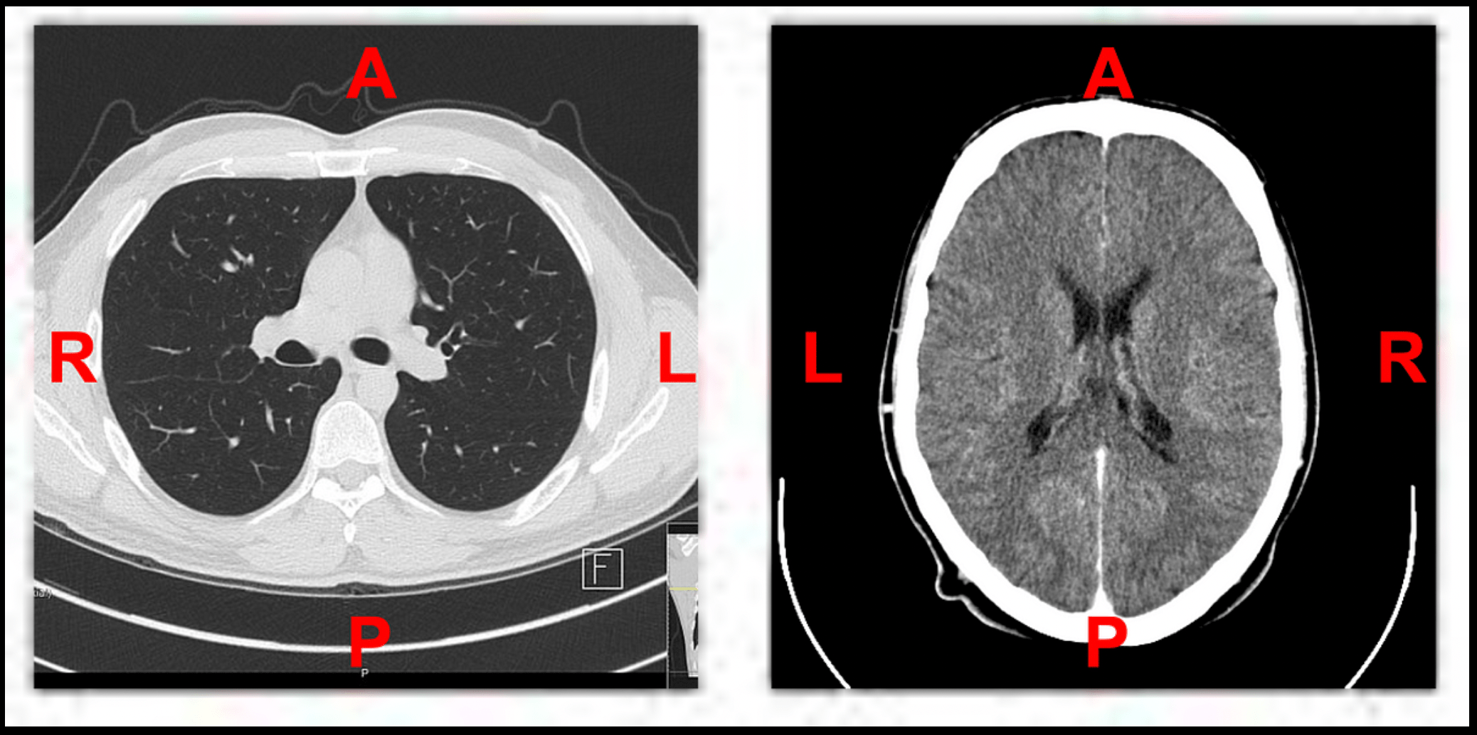
Missing or incorrect orientation tags Basic:
DICOM orientation and position tags are essential for the correct spatial display and interpretation of medical images. These tags define the relationship between the pixel data and the patient's anatomy.
- Image Orientation (Patient) (0020, 0037) : Specifies the direction cosines of the image rows and columns relative to the patient.
- Patient Position (0018, 5100) : Indicates how the patient was positioned within the scanner.
- Patient Orientation (0020, 0020) : Describes the anatomical direction of the image rows and columns.
Problem:
When these tags are missing, inconsistent, or incorrectly set during acquisition or preprocessing, images may be displayed flipped (e.g., left-right inversion) or rotated. This is critically problematic in breast imaging, where accurate laterality is mandatory.
Recommended Approach:
- Check for tags explicitly: Ensure (0020, 0037) and (0018, 5100) exist and are consistent across slices.
- Validate orientation with pixel data:
- Use libraries like SimpleITK to convert all scans to a consistent anatomical orientation using the direction cosines stored in the image headers.
Sample Code:
import os
import pydicom
import SimpleITK as sitk

def dicom_orientation_QA(folder):
    orientations = set()
    positions = set()
    lateralities = set()
    view_positions = set()

    # Iterate through DICOM files
    for f in os.listdir(folder):
        if not f.endswith(".dcm"):
            continue
        ds = pydicom.dcmread(os.path.join(folder, f))

        # Orientation & position
        orientations.add(tuple(ds.get((0x0020, 0x0037), [])))   # Image Orientation (Patient)
        positions.add(ds.get((0x0018, 0x5100), None))           # Patient Position

        # Laterality info
        lateralities.add(ds.get((0x0020, 0x0060), None))        # Laterality
        view_positions.add(ds.get((0x0018, 0x5101), None))      # View Position

    # --- Report ---
    print("=== DICOM Orientation QA Report ===")
    print(f"Unique orientations found: {orientations}")
    print(f"Unique patient positions found: {positions}")
    print(f"Unique lateralities found: {lateralities}")
    print(f"Unique view positions found: {view_positions}")

    if len(orientations) > 1:
        print(" Inconsistent Image Orientation (Patient) across slices.")
    else:
        print(" Orientation tags consistent across slices.")

    if len(positions) > 1:
        print(" Inconsistent Patient Position across slices.")
    else:
        print(" Patient Position tags consistent.")

    if len(lateralities) > 1:
        print(" Conflicting Laterality tags detected.")
    elif None in lateralities:
        print(" Missing Laterality tag.")
    else:
        print(" Laterality tags consistent.")

    if len(view_positions) > 1:
        print(" Conflicting View Position tags detected.")
    elif None in view_positions:
        print(" Missing View Position tag.")
    else:
        print(" View Position tags consistent.")

    # --- Check orientation with SimpleITK ---
    try:
        reader = sitk.ImageSeriesReader()
        dicom_names = reader.GetGDCMSeriesFileNames(folder)
        reader.SetFileNames(dicom_names)
        image = reader.Execute()
        print("SimpleITK Direction Cosines:", image.GetDirection())
    except Exception as e:
        print(" SimpleITK check failed:", e)

    print("=== End of Report ===")


def reorient_and_save(input_dicom, output_file="scan_reoriented.nii.gz"):
    image = sitk.ReadImage(input_dicom)
    # Reorient to standard anatomical orientation (RAS)
    reoriented = sitk.DICOMOrient(image, "RAS")
    sitk.WriteImage(reoriented, output_file)
    print(f" Reoriented image saved to {output_file}")


# Example Usage:
# dicom_orientation_QA("path/to/dicom/folder")
# reorient_and_save("path/to/scan.dcm")
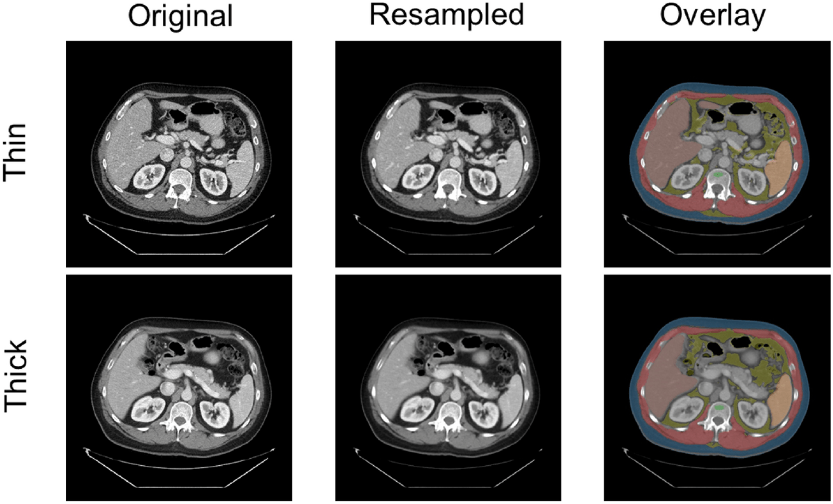
Proper resampling for dataset with mixed thin and thick slice volume 🔗
Basic:
In medical imaging, particularly with modalities like CT and MRI, spatial resolution refers to the ability to distinguish small structures that are close together, it defines how much anatomical detail can be visualized in an image. Thin slices typically offer higher spatial resolution, enhancing the visibility of fine anatomical details and small lesions. In contrast, thicker slices generally provide a better signal-to-noise ratio (SNR) and reduce image noise, but at the cost of reduced spatial resolution. The choice between thin and thick slices involves a trade-off between resolution and noise, guided by the specific clinical objectives and the anatomical region being examined.
Problem:
When working with datasets that include both thin and thick-slice volumes, inconsistency in voxel dimensions creates challenges for model training, radiomics, and visualization. This is where resampling becomes essential. Resampling involves changing voxel dimensions and the overall volume size to bring all datasets to a common resolution. Without it, variations in spatial resolution often caused by differences in scanners, protocols, or reconstruction settings may lead to bias, domain shifts, and unreliable results. Moreover, high-resolution images demand more computation, making it impractical to process large datasets efficiently. Resampling helps reduce computational complexity by increasing voxel spacing, standardizes data for consistent analysis, and improves visualization by simplifying overly detailed volumes. It also serves as a form of data compression and addresses computational limitations in real-time or resource-constrained environments.
Recommended Approach:
The most widely used technique is interpolation-based resampling. This method estimates pixel or voxel values based on neighboring data points. Common interpolation techniques include:
- Nearest neighbor: Assigns the value of the nearest pixel/voxel. This is used for labels.
- Linear interpolation: Averages the values of neighboring pixels/voxels. Provides a smoother result than nearest neighbor.
- Cubic interpolation: Uses a cubic polynomial to estimate values, offering a higher degree of smoothness and accuracy.
Additionally, resizing can be used to standardize input dimensions for deep learning models, and reformatting is helpful for generating orthogonal views (e.g., sagittal or coronal from axial stacks) through interpolation.
Example:
Sample code:
import SimpleITK as sitk

def resample_volume(image, new_spacing=(1.0, 1.0, 1.0), interpolator=sitk.sitkLinear):
    """
    Resample a 3D medical image (CT or MRI) to a specified resolution.

    Args:
        image (sitk.Image): Input image volume.
        new_spacing (tuple): Desired spacing (z, y, x) in mm.
        interpolator (SimpleITK interpolator):
            Use sitkLinear for images, sitkNearestNeighbor for labels/masks.

    Returns:
        sitk.Image: Resampled image.
    """
    original_spacing = image.GetSpacing()
    original_size = image.GetSize()

    new_size = [
        int(round(original_size[i] * (original_spacing[i] / new_spacing[i])))
        for i in range(3)
    ]

    resampler = sitk.ResampleImageFilter()
    resampler.SetOutputSpacing(new_spacing)
    resampler.SetSize(new_size)
    resampler.SetInterpolator(interpolator)
    resampler.SetOutputDirection(image.GetDirection())
    resampler.SetOutputOrigin(image.GetOrigin())
    resampler.SetDefaultPixelValue(image.GetPixelIDValue())

    return resampler.Execute(image)
import torchio as tio

def resample_volume_torchio(input_path, output_path, new_spacing=(1.0, 1.0, 1.0)):
    """
    Resample a 3D medical image using TorchIO to a specified spacing.
    Use tio.LabelMap instead of tio.ScalarImage if resampling segmentation
    masks TorchIO will automatically use nearest-neighbor interpolation for
    labels.
    Args:
        input_path (str): Path to the input image.
        output_path (str): Path to save the resampled image.
        new_spacing (tuple): Desired spacing (x, y, z) in mm.

    Returns:
        None
    """
    subject = tio.Subject(image=tio.ScalarImage(input_path))
    resampler = tio.Resample(new_spacing)
    resampled = resampler(subject)
    resampled.image.save(output_path)
Orientation normalisation before directly indexing voxel arrays or haphazardly transposing tensors 🔗
Basic:
Orientation normalization is the process of transforming a medical image volume (e.g., CT, MRI) so that it aligns with a standard anatomical frame of reference, such as LPS (Left-Posterior-Superior) or RAS (Right-Anterior-Superior). In medical image analysis, data is typically stored as 3D volumes, where voxel ordering is defined by orientation metadata. However, directly indexing voxel arrays (e.g., NumPy arrays) or arbitrarily transposing tensor dimensions without first accounting for orientation can lead to serious misinterpretations.
Problem:
Indexing voxel arrays or transposing tensors before orientation normalization can result in misaligned reference frames between volumes. This leads to incorrect anatomical interpretations, flawed spatial operations (e.g., cropping, segmentation), and ultimately invalid model outputs. Such inconsistencies are subtle and often go unnoticed during development, but they can significantly compromise model accuracy, reproducibility, and clinical reliability, especially in tasks requiring anatomical precision.
Recommended Approach:
Normalize orientation before converting medical images to NumPy arrays or tensors. This ensures consistent anatomical alignment (e.g., LPS) across subjects. Perform any image preprocessing, augmentation, or spatial operation after orientation normalization.
What NOT to do:
Don’t catch transpositis—a condition afflicting some medical imaging codebases where images get transposed multiple times until they “look right.”
Example:
Sample Code:
import SimpleITK as sitk
import numpy as np
import torch

def load_and_prepare_image(image_path, target_orientation='LPS'):
    """
    Load a medical image, normalize its orientation, and convert it to a NumPy array and PyTorch tensor.

    Args:
        image_path (str): Path to the input medical image (e.g., NIfTI or DICOM).
        target_orientation (str): Standard orientation code ('LPS' or 'RAS').

    Returns:
        numpy.ndarray: Image data as a NumPy array.
        torch.Tensor: Image data as a PyTorch tensor.
    """
    # Step 1: Load image
    image = sitk.ReadImage(image_path)

    # Step 2: Normalize orientation
    image_oriented = sitk.DICOMOrient(image, target_orientation)

    # Step 3: Convert to NumPy array
    image_array = sitk.GetArrayFromImage(image_oriented)

    # Step 4: Convert to PyTorch tensor (optional)
    image_tensor = torch.from_numpy(image_array).float()

    return image_array, image_tensor
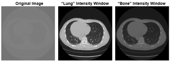
HU Clipping (and Window / Leveling) 🔗
Basic:
Hounsfield units (HU) are a dimensionless unit universally used in computed tomography (CT) scanning to express CT numbers in a standardized and convenient form. Hounsfield units are obtained from a linear transformation of the measured attenuation coefficients, which is based on the arbitrarily-assigned radiodensities of air (-1000 HU) and pure water (0 HU). HU clipping refers to enhance image quality and highlight specific tissues or structures.
Problem:
CT images contain a wide range of Hounsfield Unit (HU) values that correspond to different tissue densities, such as air, fat, soft tissue, and bone. Displaying the full HU range in a single image can reduce contrast and obscure subtle differences within specific tissues, making it harder to interpret. While CT voxels typically contain 16 bits of precision which corresponds to around 65k distinct values. The human eye and consumer grade monitors, on the other hand, can only perceive 30 to 256 levels of gray. Therefore, the original 16 bit image needs to be scaled so that humans can appropriately perceive contrast values to make appropriate clinical decisions. HU clipping addresses this by narrowing the displayed intensity range, which enhances visibility and improves tissue contrast. This is particularly beneficial for image analysis tasks like segmentation, where distinguishing between anatomical structures is essential for both human observers and machine learning algorithms. Additionally, HU clipping helps standardize the appearance of images acquired from different scanners or patients, facilitating more consistent comparisons across datasets.
Recommended Approach:
To perform HU clipping effectively, one must firstdetermine the target tissue or clinical task, such as lung, brain, or bone analysis. Based on this, an appropriate HU window can be selected to isolate the relevant intensity range. Common examples include: –1000 to 400 for lung parenchyma, –150 to 250 for soft tissue, 0 to 80 for brain structures, and 300 to 2000 for bone. Once selected, the CT intensity values are clipped to this range using tools like NumPy or SimpleITK.
Example:
A transverse slice of a chest CT with no intensity windowing, a "lung" intensity window, and a "bone" intensity window.
Sample code:
import torchio as tio

def get_torchio_hu_window_transform(hu_min: int, hu_max: int):
    """
    Returns a TorchIO transform for HU clipping and normalization to [0, 1].

    Parameters:
    ----------
    hu_min : int
        Lower HU threshold.
    hu_max : int
        Upper HU threshold.

    Returns:
    -------
    torchio.Compose
        A TorchIO Compose transform.
    """
    return tio.Compose([
        tio.ToCanonical(),
        tio.RescaleIntensity(
            out_min_max=(0, 1),
            in_min_max=(hu_min, hu_max)
        )
    ])
from monai.transforms import Compose, LoadImaged, EnsureChannelFirstd, ScaleIntensityRanged

def get_monai_hu_window_transform(hu_min: int, hu_max: int):
    """
    Returns a MONAI Compose transform for HU clipping and normalization to [0, 1].

    Parameters:
    ----------
    hu_min : int
        Lower bound of HU window.
    hu_max : int
        Upper bound of HU window.

    Returns:
    -------
    monai.transforms.Compose
        A composed MONAI transform.
    """
    return Compose([
        LoadImaged(keys=["image", "label"]),
        EnsureChannelFirstd(keys=["image", "label"]),
        ScaleIntensityRanged(
            keys="image",
            a_min=hu_min,
            a_max=hu_max,
            b_min=0.0,
            b_max=1.0,
            clip=True
        )
    ])
Labelling different contrast phases 🔗
Basic:
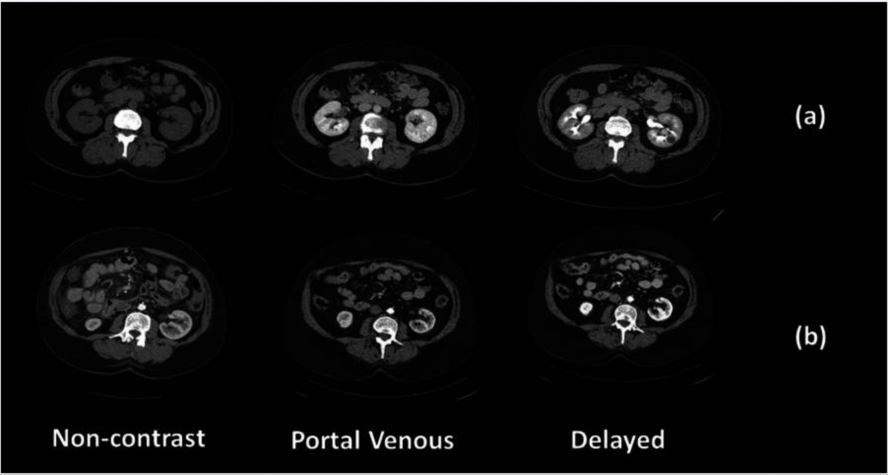
Contrast phases in CT imaging represent different time points after intravenous contrast injection, each highlighting specific tissue enhancement patterns. The contrast agent travels through the vascular system and organs, and scans are timed to capture key phases like non-contrast, portal venous, and delayed.
To identify contrast phases in CT scans using DICOM metadata, several tags are commonly referenced. TheSeries Description(0008,103E) andProtocol Name(0018,1030) often contain free-text labels like "arterial," "venous," or "delayed," which can hint at the intended phase. TheContrast/Bolus Agent(0018,0010) specifies the type of contrast used, while theContrast/Bolus Start Time(0018,1042) andSeries Time(0008,0031) orAcquisition Time(0008,0032) can be compared to estimate the delay between injection and scan
Problem:
Phase labels are often manually assigned and prone to error, especially in large datasets. Variations in contrast injection protocols, patient physiology, and scanner settings further complicate accurate labeling. Manual correction is time-consuming and inconsistent.
Recommended Approach:
- Image-Based Classification: Train a lightweight CNN or transformer-based model to classify contrast phases directly from CT images, reducing reliance on potentially incorrect metadata.
- Use Heuristics for QA: Apply simple rules based on Hounsfield Units (HU) in key regions (e.g., liver, aorta) to flag likely mislabels.
- Time-Based Sorting (if multi-phase scans are present): Use DICOM metadata such as Acquisition Time to infer the chronological order of phases (e.g., non-contrast < portal venous < delayed).
- Robust Labeling Pipeline: Store phase predictions separately (e.g., JSON/CSV) rather than overwriting source data. Allow human review for uncertain cases.
Example:
Sample Code:
This function estimates the CT contrast phase (Non-contrast, Arterial, Venous, Delayed) based on the average intensity of an image series.
## ⚡ Simple Contrast Phase Detection Based on Mean HU Values

```python
import numpy as np

def detect_contrast_phase(image_series):
    """
    Estimate contrast phase using mean HU value of the entire image series.

    Parameters:
    -----------
    image_series : np.ndarray
        A NumPy array representing a CT volume or series of slices (in HU).

    Returns:
    --------
    str
        Estimated phase: 'NC' (Non-contrast), 'ART' (Arterial),
                         'VEN' (Venous), or 'DEL' (Delayed).
    """
    mean_hu = np.mean(image_series)
    std_hu = np.std(image_series)

    if mean_hu < 50:
        return "NC"
    elif 50 <= mean_hu < 90:
        return "ART"
    elif 90 <= mean_hu < 120:
        return "VEN"
    else:
        return "DEL"
Using ECG/respiratory gating information in cardiac CT 🔗
Basic:
Cardiac CT imaging captures the anatomy and function of the heart, which is a moving organ. To reduce motion artifacts caused by the cardiac cycle and breathing, CT systems use ECG gating and, less commonly, respiratory gating. Cardiac gating or ECG-gated angiography in CT is an acquisition technique that triggers a scan during a specific portion of the cardiac cycle. Often, this technique is used to obtain high-quality scans void of pulsation artifact. These gating signals are often recorded in the DICOM metadata or as auxiliary files.
In cardiac CT imaging, DICOM tags related to ECG and respiratory gating provide crucial metadata for understanding when in the physiological cycle each image was acquired. Key tags includeCardiac Reconstruction Phase(0018,9152), which indicates the percentage of the R–R interval (e.g., 75% for end-diastole), andTrigger Time(0018,1060), which specifies the time offset from the ECG R-wave. Additional tags such asHeart Rate(0018,1088),Gating Type(0018,1031), andTrigger Source(0018,1061) describe how and whether ECG or respiratory gating was applied. These tags are essential for selecting motion-minimized frames, ensuring phase consistency in datasets, and enabling accurate downstream analysis in both clinical and AI workflows.
Problem:
Ignoring ECG or respiratory gating information in cardiac CT can result in using frames affected by motion, leading to degraded image quality and poor diagnostic utility. In AI pipelines, training or inference on ungated or incorrectly phased images can reduce model performance, especially for tasks like coronary calcium scoring, left ventricular segmentation, or functional analysis. Furthermore, not accounting for gating can lead to inconsistencies when comparing multi-phase datasets or across subjects, where different cardiac phases may have been captured. This undermines reproducibility, accuracy, and generalizability of downstream analysis.
Recommended Approach:
- Identify and extract image series closest to a specific cardiac phase (e.g., 75% R–R interval for end-diastole).
- For AI pipelines, train only on motion-minimized gated phases, or include phase as a metadata variable.
- If multiple phases are available (e.g., 10-frame cine CT), select or average phases after quality assessment.
- Consider frame rejection strategies using variance or artifact detection if explicit gating info is missing.
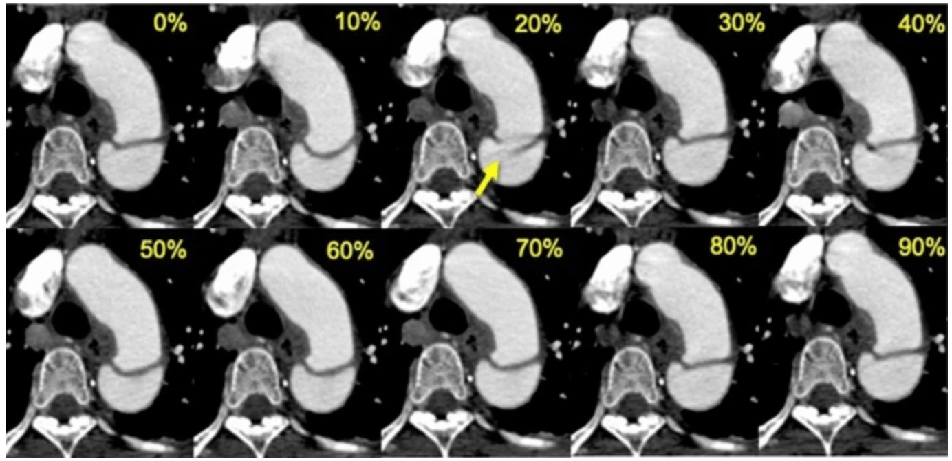
Example:
Images comparing retrospective ECG-gated CT angiography at each phase of the R-R interval in a 53-year-old man with acute aortic dissection
Sample Code:
This Python function scans a folder of ECG-gated cardiac CT DICOM files and selects the slice closest to a specified cardiac phase (e.g., 75% of the R–R interval).
import pydicom
import numpy as np
from pathlib import Path

def analyze_cardiac_gating(dicom_folder, target_phase=75):
    """
    Analyze ECG-gated cardiac CT series and select images closest to target cardiac phase.

    Args:
        dicom_folder: Path to folder containing DICOM files
        target_phase: Desired cardiac phase (% of R-R interval, typically 70-75% for end-diastole)

    Returns:
        Dictionary containing gating information and selected slices
    """
    dicom_files = list(Path(dicom_folder).glob('*.dcm'))
    if not dicom_files:
        raise FileNotFoundError("No DICOM files found in the specified folder")

    # Collect gating info from all slices
    gating_data = []
    for file in dicom_files:
        ds = pydicom.dcmread(file)

        try:
            phase = float(ds.CardiacReconstructionPhase)  # (0018,9152)
            trigger_time = float(ds.TriggerTime) if 'TriggerTime' in ds else None  # (0018,1060)
            heart_rate = float(ds.HeartRate) if 'HeartRate' in ds else None  # (0018,1088)

            gating_data.append({
                'file': file,
                'phase': phase,
                'trigger_time': trigger_time,
                'heart_rate': heart_rate,
                'instance_number': int(ds.InstanceNumber)
            })
        except AttributeError as e:
            print(f"Missing gating tags in {file.name}: {e}")
            continue

    if not gating_data:
        raise ValueError("No valid ECG-gated DICOM files found")

    # Find slice closest to target phase
    phases = np.array([x['phase'] for x in gating_data])
    phase_diffs = np.abs(phases - target_phase)
    best_idx = np.argmin(phase_diffs)
    best_slice = gating_data[best_idx]


    return {
        'best_slice': best_slice,
        'all_slices': sorted(gating_data, key=lambda x: x['instance_number'])
    }
Handling vendor-specific header inconsistencies 🔗
-
Critical parameters hidden in vendor-specific private tags Basic:
Medical imaging vendors often use different conventions and private DICOM tags for storing metadata, even when the imaging modality (e.g., CT, MRI) is the same. While the DICOM standard defines many core attributes, manufacturers frequently insert vendor-specific extensions, nonstandard names, or omit expected fields altogether. This creates variation across scanners from GE, Siemens, Philips, Canon, etc.
Problem:
Hardcoding data loaders or preprocessing pipelines to expect fixed tag names or structures can result in failures when encountering data from a different vendor. For example, one scanner may store series description under standard tags, while another may embed important phase or orientation info in private tags or use different encodings. As a result, such rigid pipelines may miss key metadata, misinterpret orientations, or even crash during parsing. This creates poor generalizability, especially when scaling to multi-center datasets or deploying models across institutions.
Recommended Approach:
- Identify manufacturer (0008,0070) early in processing
- Identify private tags using the DICOM dictionary: standard tags have known names, while private tags typically show up as (gggg, xxxx) with odd group numbers or unknown VR.
- Use vendor documentation or site-specific knowledge to interpret them.
- For cross-vendor workflows, rely primarily on standard DICOM attributes and use private tags only when absolutely necessary.
Sample Code:
import os import pydicom from pydicom.tag import Tag def extract_series_description(ds): """Extracts series description with vendor-specific fallback.""" if hasattr(ds, "SeriesDescription"): return ds.SeriesDescription # Standard tag (0008,103E) # Example vendor-specific private tag fallback private_tag = Tag(0x0009, 0x1010) if private_tag in ds: return str(ds[private_tag].value) return "Unknown" def detect_vendor(ds): """Identify scanner vendor from tag (0008,0070).""" return getattr(ds, "Manufacturer", "Unknown") def load_dicom_headers(folder_path): """Parse headers with vendor-aware fallbacks and validation.""" files = [f for f in os.listdir(folder_path) if f.lower().endswith(".dcm")] for file in files: filepath = os.path.join(folder_path, file) try: ds = pydicom.dcmread(filepath, stop_before_pixels=True) vendor = detect_vendor(ds) desc = extract_series_description(ds) print(f"{file} → Vendor: {vendor} | Series: {desc}") except Exception as e: print(f"Error reading {file}: {e}") # Example usage # load_dicom_headers("path/to/dicom_folder") -
Manufacturer-specific pixel padding Basic:
Pixel padding is the practice of assigning a uniform value to pixels outside the scanned field of view. Pixel Padding Value (0028,0120) is typically used to pad grayscale images (those with a Photometric Interpretation (0028,0004) of MONOCHROME1 or MONOCHROME2), or color images with a Photometric interpretation (0028,0004) of PALETTE COLOR, to rectangular format. However, vendors may implement it inconsistently, sometimes using zeros, large negative numbers, or undocumented private values.
Problem:
Different manufacturers may use different padding values (e.g., 0, -1024, -2000, -32768) and may not always populate the Pixel Padding Value tag. This inconsistency can lead to background padding being mistaken for valid anatomy, skewing intensity-based analyses (e.g., histograms, segmentation thresholds) and introducing artifacts into quantitative workflows.
Recommended Approach:
- Check for Pixel Padding Value tag: Use
(0028,0120)and(0028,0121)to identify the padding value and range, if available. - Mask out padding:
- Create a binary mask where pixels equal to the padding value are excluded.
Example:
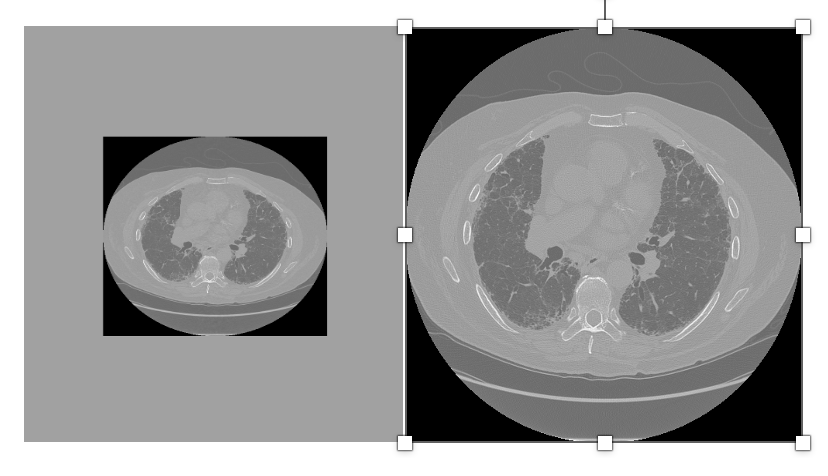
Image with padding Image after removing the padding
Sample Code:
import pydicom import numpy as np def load_image_without_padding(dicom_path): ds = pydicom.dcmread(dicom_path) pixel_array = ds.pixel_array.astype(np.int16) # Try to get padding value from DICOM tags padding_value = getattr(ds, 'PixelPaddingValue', None) if padding_value is None: # Heuristic: assume values lower than -1000 are padding (for CT) padding_value = -32768 if np.min(pixel_array) < -1000 else None if padding_value is not None: mask = (pixel_array != padding_value) cleaned_array = np.where(mask, pixel_array, np.nan) else: cleaned_array = pixel_array return cleaned_array # Usage image = load_image_without_padding("ct_scan.dcm") - Check for Pixel Padding Value tag: Use
Avoiding Spatial Errors: Evaluating Metrics in Scanner vs. Patient Space 🔗
Basic:
In medical image analysis, particularly with CT or MRI data, images are typically stored in one of two coordinate systems: scanner (or voxel) space and patient (or world) space.
Scanner Space (or Image Space): This refers to the coordinate system defined by the scanner itself during image acquisition. It's the physical space within the scanner where the data is collected.
Patient Space: This refers to the anatomical coordinate system of the patient, often defined by anatomical landmarks or a reference coordinate system.
Problem:
Computing spatial metrics or alignment-based evaluations in scanner space without accounting for the physical voxel spacing, image origin, and orientation can introduce significant errors. For example, comparing a segmentation mask in patient space (with correct spatial alignment) to one in scanner space (just voxel-aligned) may falsely report poor overlap or boundary accuracy. This can mislead model performance evaluation, especially in multi-scanner or multi-center datasets where spacing and orientation vary.
Recommended Approach:
Convert both predicted and ground-truth masks to the same space before comparison, ideally to patient space using DICOM/SITK orientation metadata.
Sample code:
import SimpleITK as sitk
import numpy as np
from typing import Tuple, Dict

class SpaceAwareEvaluator:
    """
    Handles spatial metrics computation while maintaining awareness of coordinate spaces.
    Converts all inputs to patient space before evaluation.
    """

    def __init__(self, reference_image: sitk.Image):
        """
        Initialize with a reference image that defines the target patient space.

        Args:
            reference_image: sitk.Image with proper patient space metadata
        """
        self.reference_space = reference_image
        self.metrics = {}

    def _ensure_patient_space(self, image: sitk.Image) -> sitk.Image:
        """Convert image to patient space if not already"""
        if not self._is_in_patient_space(image):
            return self._transform_to_patient_space(image)
        return image

    def _is_in_patient_space(self, image: sitk.Image) -> bool:
        """Check if image shares patient space with reference"""
        return (
            np.allclose(image.GetOrigin(), self.reference_space.GetOrigin()) and
            np.allclose(image.GetSpacing(), self.reference_space.GetSpacing()) and
            np.allclose(image.GetDirection(), self.reference_space.GetDirection())
        )

    def _transform_to_patient_space(self, image: sitk.Image) -> sitk.Image:
        """Resample image to reference patient space"""
        return sitk.Resample(
            image,
            self.reference_space,
            sitk.Transform(),
            sitk.sitkNearestNeighbor,  # For masks/labels
            0,  # Default background value
            image.GetPixelID()
        )

    def compute_metrics(
        self,
        prediction: sitk.Image,
        ground_truth: sitk.Image,
        metric_names: list = ['dice', 'hausdorff', 'surface_distance']
    ) -> Dict[str, float]:
        """
        Compute spatial metrics after ensuring both images are in patient space.

        Args:
            prediction: Segmentation mask (scanner or patient space)
            ground_truth: Reference mask (scanner or patient space)
            metric_names: List of metrics to compute

        Returns:
            Dictionary of metric names and values
        """
        # Convert both images to patient space
        pred_patient = self._ensure_patient_space(prediction)
        gt_patient = self._ensure_patient_space(ground_truth)

        # Compute requested metrics
        results = {}
        if 'dice' in metric_names:
            overlap_filter = sitk.LabelOverlapMeasuresImageFilter()
            overlap_filter.Execute(gt_patient, pred_patient)
            results['dice'] = overlap_filter.GetDiceCoefficient()

        if 'hausdorff' in metric_names or 'surface_distance' in metric_names:
            hausdorff_filter = sitk.HausdorffDistanceImageFilter()
            hausdorff_filter.Execute(gt_patient, pred_patient)
            results['hausdorff'] = hausdorff_filter.GetHausdorffDistance()

            if 'surface_distance' in metric_names:
                results['surface_mean'] = hausdorff_filter.GetAverageHausdorffDistance()

        return results

# Usage Example
if __name__ == "__main__":
    # Load images (example paths)
    reference_ct = sitk.ReadImage("path/to/reference_ct.dcm")
    scanner_space_mask = sitk.ReadImage("path/to/scanner_space_mask.nii.gz")
    patient_space_mask = sitk.ReadImage("path/to/patient_space_mask.nii.gz")

    # Initialize evaluator with reference CT (defines desired patient space)
    evaluator = SpaceAwareEvaluator(reference_ct)

    # Compute metrics - handles space conversion automatically
    metrics = evaluator.compute_metrics(
        prediction=scanner_space_mask,
        ground_truth=patient_space_mask,
        metric_names=['dice', 'hausdorff']
    )

    print(f"Dice Coefficient: {metrics['dice']:.3f}")
    print(f"Hausdorff Distance: {metrics['hausdorff']:.2f} mm")
Using random-seed control to produce experiments 🔗
Basic:
Random seeds are used to control the pseudo-random number generators (PRNGs) in machine learning experiments. This includes operations such as data splitting, weight initialization, data augmentation, and shuffling.
Problem:
Omitting seed control causes:
- Non-reproducible results : Different runs yield varying metrics despite identical code/hyperparameters
- Unreliable comparisons : Cannot fairly evaluate model improvements
- Debugging challenges : Inconsistent behavior masks implementation errors
- Scientific integrity risks : Published results become non-verifiable
Recommended Approach:
Set random seeds explicitly for all randomness sources: Python, NumPy, and deep learning frameworks like PyTorch or TensorFlow and store it in experiment metadata or logging tools.
Sample Code:
import random
import numpy as np
import torch

def set_seed(seed=42):
    random.seed(seed)
    np.random.seed(seed)
    torch.manual_seed(seed)
    torch.cuda.manual_seed_all(seed)

    # For deterministic behavior
    torch.backends.cudnn.deterministic = True
    torch.backends.cudnn.benchmark = False

set_seed(42)
Not relying on default nnU-Net post-processing when class imbalance 🔗
Basic:
nnU-Net includes automatic post-processing, such as connected component analysis, to clean up predictions (e.g., keeping only the largest connected component). While these defaults are effective for many tasks, they are not universally optimal, especially in multi-class or class-imbalanced settings.
Problem:
When using default post-processing, nnU-Net may remove small but clinically significant structures (e.g., small tumors or vessels) from underrepresented classes. This disproportionately affects rare classes, leading to reduced recall and distorted performance metrics. In extreme cases, entire classes may be missed if their components are smaller than the largest background-connected region.
Recommended Approach:
Develop and integrate custom post-processing logic that uses class-specific thresholds for preserving smaller, significant structures.
Example Image:
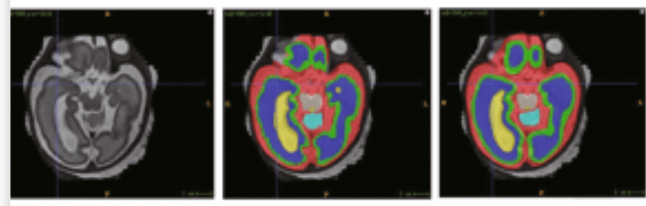
Original Image Ground Truth nnU-Net
Sample Code:
This can be done by overriding the remove_all_but_largest_component() logic in nnU-Net’s postprocessing pipeline.
from nnunet.postprocessing.connected_components import load_remove_save

# Override the default CCA
def new_remove_all_but_largest_component(binary_image: np.ndarray, *args, **kwargs):
    min_sizes = {1: 50, 2: 20}  # Class-specific thresholds
    class_idx = kwargs.get('class_idx', 1)  # Pass class index from load_remove_save
    return custom_cca(binary_image, class_idx, min_sizes)

# Replace nnU-Net's function
import nnunet.postprocessing.connected_components as orig_cca
orig_cca.remove_all_but_largest_component = new_remove_all_but_largest_component
Not neglecting anisotropic z-spacing when selecting 3-D kernels and strides 🔗
Basic:
In 3D medical imaging (e.g., CT or MRI), voxel dimensions are not always uniform in all directions. This is particularly true in the z-axis (slice direction), which often has a larger spacing than the x and y dimensions. This non-uniformity is called anisotropic spacing. When applying 3D convolutions or downsampling operations, ignoring this anisotropy can lead to inappropriate kernel sizes and strides, potentially degrading model performance.
Problem:
When 3D kernels or strides are selected without accounting for anisotropic z-spacing, it can lead to many problems:
- Difficulty in learning meaningful features: Standard 3x3x3 isotropic kernels might struggle to learn effectively from anisotropic voxels due to varying information density along each dimension.
- Missing important information: If strides in the z-direction are chosen to be large, important information between slices can be skipped, especially in tasks like detection where subtle details are crucial.
Recommended Approach:
- Use anisotropic kernels for initial layers, e.g., (1×3×3) instead of (3×3×3), to limit operations in the z-direction when spacing is large, at least in initial layers.
- Resampling the image to isotropic resolution to compensate for anisotropic spacing however it can introduce redundant data, leading to unnecessary computational cost.
Sample Code:
import torch.nn as nn

class Anisotropic3DCNN(nn.Module):
    def __init__(self):
        super().__init__()
        # Early layer: Avoid downsampling in Z
        self.conv1 = nn.Conv3d(1, 16, kernel_size=(1, 3, 3), stride=(1, 2, 2), padding=(0, 1, 1))
        self.bn1 = nn.BatchNorm3d(16)
        self.relu1 = nn.ReLU()

        # Later layer: Isotropic kernel (Z is more meaningful now)
        self.conv2 = nn.Conv3d(16, 32, kernel_size=(3, 3, 3), stride=(2, 2, 2), padding=1)
        self.bn2 = nn.BatchNorm3d(32)
        self.relu2 = nn.ReLU()

    def forward(self, x):
        x = self.relu1(self.bn1(self.conv1(x)))
        x = self.relu2(self.bn2(self.conv2(x)))
        return x
Not committing checkpoints larger than 1 GB directly to Git 🔗
Basic:
Large model checkpoints, especially those from deep learning frameworks like PyTorch or TensorFlow, can exceed several gigabytes in size.
Problem:
Developers sometimes try to commit these files directly to Git, unaware that Git is not optimized for large binary files.
Recommended Approach:
Git LFS (Large File Storage)
- Stores large files externally (on GitHub/GitLab servers) while keeping pointers in Git
- Best for checkpoints that change frequently but are needed by all team members
Sample Code:
# Install Git LFS
git lfs install

# Track checkpoint files
git lfs track "*.ckpt" "*.h5" "*.pth"

# Commit as usual (LFS handles the rest)
git add .gitattributes
git add model.ckpt
git commit -m "Add model checkpoint"
Compression and Storage Issues 🔗
-
JPEG2000 Lossy compression Basic:
Medical images are often compressed for storage and transmission. JPEG2000 supports both lossless and lossy compression. Lossless compression preserves pixel intensities exactly, while lossy compression discards subtle details to achieve higher compression ratios.
The DICOM Transfer Syntax UID (0002,0010) is a mandatory Data Element in the File Meta Information that identifies the specific encoding rules and format used for the dataset, such as byte order (endianness) and whether VR (Value Representation) is implicit or explicit. This identifier is essential for a DICOM viewer or processor to correctly interpret the file's encoded data. It must be located within the file's meta information and is not allowed to appear anywhere else within the dataset itself.
Problem:
- Lossy JPEG2000 may blur or smooth out tiny lesions, calcifications, or lung nodules.
- It can introduce quantitative bias in radiomics or AI models that rely on precise pixel intensities.
- Once saved in lossy mode, the original image fidelity cannot be recovered.
Recommended Approach:
- Prefer lossless storage for diagnostic and AI workflows.
- Detect compression type by checking DICOM Transfer Syntax UID (0002,0010).
- Flag lossy datasets before use in quantitative analysis.
Sample Code:
import pydicom
import SimpleITK as sitk

def check_and_convert_compression(dicom_file, out_file="output.nii.gz"):
    ds = pydicom.dcmread(dicom_file, stop_before_pixels=True)
    ts_uid = ds.file_meta.TransferSyntaxUID

    lossy_uids = {
        "1.2.840.10008.1.2.4.91": "JPEG2000 Lossy",
        "1.2.840.10008.1.2.4.81": "JPEG-LS Lossy",
        "1.2.840.10008.1.2.4.50": "JPEG Baseline (Lossy)"
    }

    if str(ts_uid) in lossy_uids:
        print(f" Image uses {lossy_uids[str(ts_uid)]}")
    else:
        print(" Image is lossless")

    # Convert to lossless NIfTI for downstream use
    image = sitk.ReadImage(dicom_file)
    sitk.WriteImage(image, out_file)
    print(f"Image saved in lossless format: {out_file}")

# Example usage
check_and_convert_compression("example.dcm")
AI/ML Specific Pitfalls 🔗
-
Reconstructed screenshots instead of raw pixel data Basic:
In medical imaging, a secondary capture is essentially a screenshot or re-rendering of an image, rather than the original raw acquisition data. These captures are typically stored as DICOMs but lack the quantitative fidelity of the source images. For example, a secondary capture might include annotations, overlays, burned-in text, or compressed pixel intensities.
Problem:
A major issue arises when secondary captures are inadvertently mixed with original imaging data in AI/ML pipelines. Since they look like valid DICOM images but are actually derived screenshots, they can mislead algorithms into learning features that do not represent true anatomy or pathology. For instance, a model may learn to detect burned-in annotations or pixel artifacts instead of clinical findings. Moreover, secondary captures often lack essential metadata such as accurate pixel spacing, modality-specific acquisition parameters, and raw intensity values. This not only reduces the reproducibility of experiments but also compromises the generalizability of trained models across institutions. Ultimately, training on secondary captures can result in models that fail when deployed in real-world clinical settings where only raw acquisitions are present.
Recommended Approach:
To mitigate this issue, it is important to explicitly detect and exclude secondary captures before training or inference. Secondary captures can be identified using DICOM metadata, particularly the SOP Class UID (0008, 0016) and the Secondary Capture Image Storage class (
1.2.840.10008.5.1.4.1.1.7). Pipelines should be designed to automatically filter out these instances to prevent them from contaminating the dataset. Additionally, validating images with modality tags (0008, 0060) and checking for acquisition-specific attributes (such as pixel spacing (0028, 0030) and rescale parameters) can help ensure that only raw acquisitions are included. By systematically excluding secondary captures, one can maintain dataset integrity and improve the reliability of AI models across diverse clinical environments.Sample Code:
import os import pydicom def is_secondary_capture(dicom_ds): """Check if a DICOM is a secondary capture.""" sop_class_uid = dicom_ds.get((0x0008, 0x0016), None) if sop_class_uid and sop_class_uid.value == "1.2.840.10008.5.1.4.1.1.7": return True return False def filter_dicom_folder(folder_path): valid_files = [] secondary_captures = [] for root, _, files in os.walk(folder_path): for f in files: if f.lower().endswith(".dcm"): try: ds = pydicom.dcmread(os.path.join(root, f), stop_before_pixels=True) if is_secondary_capture(ds): secondary_captures.append(f) else: valid_files.append(f) except Exception as e: print(f"Skipping {f}: {e}") return valid_files, secondary_captures # Example usage dicom_folder = "path/to/dicom_dataset" valid, secondary = filter_dicom_folder(dicom_folder) print("Valid raw acquisitions:", len(valid)) print("Excluded secondary captures:", len(secondary)) -
Mixing modalities with similar appearance Basic:
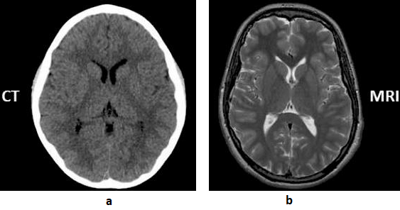
CT (Computed Tomography) scans use X-rays for fast, detailed images of bones and organs, making them ideal for emergency situations and detecting acute injuries like fractures or bleeding. MRI (Magnetic Resonance Imaging) uses magnets and radio waves for superior, high-detail imaging of soft tissues, brain, spinal cord, ligaments, and organs.
A contrast-enhanced CT scan is when a contrast agent (typically iodine-based) is injected into a patient’s bloodstream, usually through an IV line, during the scanning procedure. The contrast agent contains substances that absorb X-rays differently from surrounding tissues, making blood vessels, organs and abnormalities more visible on the CT images. As the contrast agent circulates through the body, it highlights blood vessels and other structures, enhancing their visibility on the images.
Unlike contrast-enhanced CT scans, which involve the injection of a contrast into the bloodstream to highlight certain structures or abnormalities, a non-contrast CT scan is performed without the use of any intravenous contrast.
The Modality tag (0008,0060) in the DICOM standard describe type of device, process or method that originally acquired the data used to create the Instances in this Series.
Problem:
In clinical imaging workflows, different modalities and scan types may appear visually similar, which can lead to mislabeled or misclassified DICOM data. This creates risks in automated pipelines, research datasets, and even diagnostic interpretation.
- CT vs MR scout/localizer images: Scout or localizer images can resemble simple projection images, making it difficult to distinguish whether they originate from CT or MRI.
- Some AI tasks explicitly require separation of contrast vs non-contrast (e.g.,
- Hemorrhage detection → requires non-contrast CT only.
- CT angiography (CTA) vessel analysis → requires contrast CT.
If mislabeled scans slip in:
- A “hemorrhage detection” model might get trained on contrast scans, where vessels look like hyperdense blood.
- An “aneurysm detection” model trained on non-contrast CT won’t see vessels properly, leading to false negatives.
Recommended Approach:
- Validate the Modality tag (0008, 0060) to ensure CT and MRI images are not mixed.
- Distinguish scout/localizer images using the Image Type (0008, 0008) or Series Description (0008, 103E).
- For contrast scans, check Contrast/Bolus Agent (0018, 0010) and related contrast usage tags.
Example:
Sample Code:
import os import pydicom def check_modality_and_contrast(folder): for f in os.listdir(folder): if not f.endswith(".dcm"): continue ds = pydicom.dcmread(os.path.join(folder, f)) modality = ds.get((0x0008, 0x0060), "Unknown") series_desc = ds.get((0x0008, 0x103E), "Unknown") image_type = ds.get((0x0008, 0x0008), []) contrast = ds.get((0x0018, 0x0010), None) print(f"File: {f}") print(f" Modality: {modality}") print(f" Series Description: {series_desc}") print(f" Image Type: {image_type}") print(f" Contrast Agent: {contrast}") # Checks if modality not in ["CT", "MR"]: print(" Unexpected modality, review required.") if "SCOUT" in str(series_desc).upper() or "LOCALIZER" in str(series_desc).upper(): print(" Scout/Localizer detected, exclude from diagnostic dataset.") if contrast is None and "CONTRAST" in str(series_desc).upper(): print(" Contrast study suspected but no Contrast/Bolus Agent tag found.") # Example usage check_modality_and_contrast("path/to/dicom_folder") -
Label leakage via DICOM metadata Basic:
Label leakage (also known as target or data leakage) occurs when information that would not realistically be available at prediction time is inadvertently included in a model’s training data. This leads to overly optimistic performance during validation but poor generalization in real-world use.
In medical imaging, this problem often arises from DICOM (Digital Imaging and Communications in Medicine) metadata. While the intended goal is to train models that recognize disease-relevant patterns from image pixels, DICOM headers frequently contain rich contextual information. Fields such as Laterality (0020,0060), Study Description (0008,1030), or Accession Number (0008,0050) may directly or indirectly encode diagnostic labels (e.g., “Left Lung Cancer” written in the description, or accession numbers systematically linked to positive cases). When this happens, models can exploit metadata “shortcuts” instead of learning meaningful image-based features.
Problem:
- Models may achieve artificially inflated accuracy by learning from metadata instead of images.
- Results become non-generalizable, failing in real clinical deployment where metadata is anonymized, inconsistent, or unavailable.
- Introduces research bias, leading to irreproducible studies.
Recommended Approach:
- Only include metadata that is clinically justified and available at inference time.
- Pass metadata explicitly as structured inputs if required, rather than hidden inside filenames or headers.
Sample Code:
import pydicom
import os

# Tags that often leak ground truth
SENSITIVE_TAGS = [
    ("0020","0060"),  # Laterality
    ("0008","1030"),  # Study Description
    ("0008","0050"),  # Accession Number
]

def strip_sensitive_tags(dicom_path, save_path=None):
    ds = pydicom.dcmread(dicom_path)

    for tag in SENSITIVE_TAGS:
        if tag in ds:
            print(f"[INFO] Removing {tag}: {ds[tag].value}")
            del ds[tag]

    if save_path:
        ds.save_as(save_path)
    return ds

# Example usage
cleaned = strip_sensitive_tags("patient_study.dcm", "patient_study_cleaned.dcm")
Revision History 🔗
| Date | Changes |
|---|---|
| 2025-07-15 | Initial Version |