Introduction 🔗

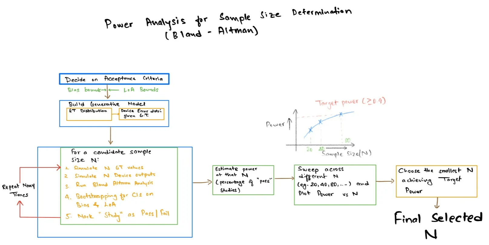
This guide will show you how to use a simulation to approximate the required sample size for a method comparison study when your pass or fail criterion is specified in terms of Bland Altman Limits of Agreement (LoA). The aim is to find the smallest sample size $N$ for which there is a high chance (power) of passing pre-specified acceptance criteria for bias and LoA , assuming realistic values for patient physiology (ground truth) and measurement error. Since acceptance criteria for LoA are expressed with confidence intervals, commonly via bootstrapping, the explicit power equations are often difficult to derive or do not exist. So we resort to simulation where we simulate many artificial studies with $N $ patients, calculate Bland Altman statistics with confidence intervals, check the acceptance criteria and then see what fraction of simulated studies “pass”. Sweeping $N$ produces a power curve that helps to make a reasonable choice for verification and validation planning.
Implementation Walkthrough 🔗
Step 1 : Define the ground truth distribution 🔗
We start by simulating the distribution of the true physiological variable in our intended use population (the reference measurement that we are going to validate against). The distribution is a representation of the patients that we are going to include in our Validation and Verification (V&V) trial, so we want it to be based on the literature, a previous study, or a small pilot measurement set. For purposes of a rough sanity check, we might simulate a large number of samples from a normally distributed variable with mean and standard deviation. If it is a bounded variable (like ratios), we use a corresponding bounded distribution to prevent us from simulating nonsensical values.
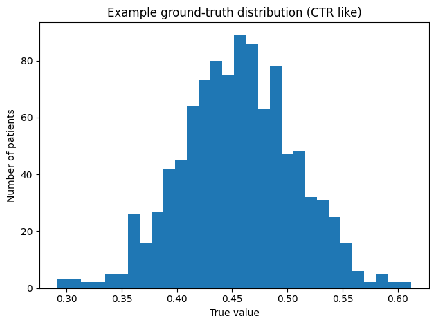
Worked example (CTR) : In our example, we use the Cardiothoracic Ratio (CTR). We chose a mean value of the ground truth distribution of μ = 0.46, which is roughly what we predicate in our previous article (cite ref article). For the spread of our ground truth we choose σ = 0.05, which is a starting point for illustration purposes, but it should be replaced in practice with values from literature, experts review, historical or pilot studies on the population of interest. We quickly validate our choice by simulating 1000 patients, which we plot as histogram (Fig. below)
# Importing libraries
import numpy as np
import matplotlib.pyplot as plt
import pandas as pd
'''
In our example lets assume that the true CTR in the population follows a normal
distribution with this mean and standard deviation.
'''
mean_true_ctr = 0.46
std_true_ctr = 0.05

# Let's draw 1000 "true" values to see what this looks like
n_demo = 1000
true_values = np.random.normal(mean_true_ctr, std_true_ctr, size=n_demo)
true_values = np.clip(true_values, 0.0, 1.0) # To make it bounded distribution
#Histogram visulation of the Ground Truth
plt.figure()
plt.hist(true_values, bins=30)
plt.xlabel("True value")
plt.ylabel("Number of patients")
plt.title("Example ground-truth distribution (CTR-like)")
plt.tight_layout()
Step 2 : Model device behavior 🔗
For each simulated patient $i$, you already have a ground truth (reference) value $x_i$, from Step 1. In Step 2, we simulate a result from the device (or algorithm) , denoted by $y_i$, on the basis of a measurement error model given $x_i$. This error model is our expectation of a performance during V&V. It is not intentionally modeling how the algorithm is supposed to operate but is a statistical approximation of the error we might see when comparing algorithm results to the reference standard.
A common, simple starting point is the additive bias plus noise model :
\[y_i = x_i + b + \varepsilon_i, \qquad \varepsilon_i \sim \mathcal{N}(0,\sigma_\varepsilon^2)\]where $b$ is the expected systematic bias (the degree to which the device is expected to over or underestimate) and $\sigma_\varepsilon$ is used to control the random error (precision).
If you suspect performance changes with the magnitude of the measurement, you can extend this to a proportional or affine model , for example :
\(y_i = x_i + b + \varepsilon_i\) or \(\sigma_\varepsilon(x_i) = \sigma_0 + k\,x_i\)
The challenge is to make the best selections for $b$, $\sigma$ and other factors based on the best available evidence, such as pilot results, known performance of existing devices, etc. In practice, it is often useful to define multiple scenarios (optimistic / nominal / pessimistic) and run the full sample size simulation under each to understand how sensitive required N is to performance assumptions.
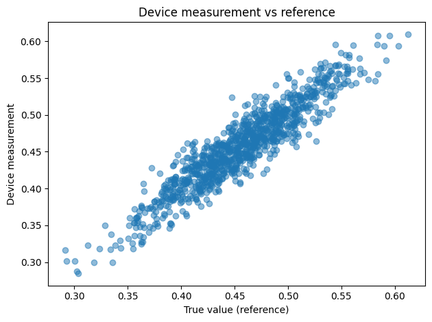
In our example case, we validate the device model with quick visuals :
- Scatter plot of the device output y with respect to the reference value x in order to check that the relationship appears reasonable.
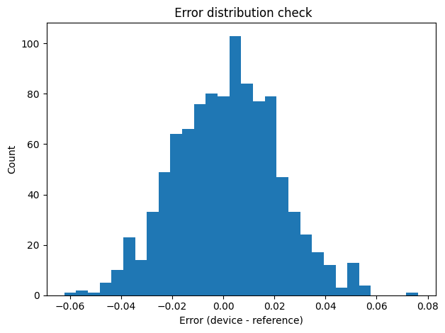
- Histogram of the error $d_i = y_i - x_i$ to check whether the presumed distribution of errors is reasonable (for instance, whether it is approximately normal shaped, or heavily tailed with outliers).
These checks help to stop unrealistic assumptions early, before we move on to calculating the Bland Altman statistics and the power for the acceptance criteria.
'''
Lets define how the device is behaving assuming the device measurement is the
true value.
'''
device_bias = 0.001      # small systematic bias
device_sd = 0.02         # random error

def simulate_device_measurements(true_vals, bias, sd):
    """Return device readings = true values + bias + noise."""
    noise = np.random.normal(bias, sd, size=len(true_vals))
    return true_vals + noise

device_values = simulate_device_measurements(true_values, device_bias, device_sd)

# Scatterplot: device vs reference to see the relationship
plt.figure()
plt.scatter(true_values, device_values, alpha=0.5)
plt.xlabel("True value (reference)")
plt.ylabel("Device measurement")
plt.title("Device measurement vs reference")
plt.tight_layout()
errors = device_values - true_values

plt.figure()
plt.hist(errors, bins=30)
plt.xlabel("Error (device - reference)")
plt.ylabel("Count")
plt.title(" Error distribution check")
plt.tight_layout()
Step 3 : Translate acceptance criteria into number 🔗
Now that we can simulate paired measurements $(x_i, y_i)$, we require numeric acceptance criteria that state what “pass” means in the context of a Bland Altman analysis. For numeric results, acceptance criteria typically consider the following :
- Bias : The mean difference
- Differences and SD : \(d_i = y_i - x_i, \qquad s_d = \mathrm{SD}(d_1,\ldots,d_N)\)
- Limits of Agreement (LoA) :
\(\text{LoA}_{\text{lower}} = \bar{d} - 1.96\, s_d, \qquad\text{LoA}_{\text{upper}} = \bar{d} + 1.96\, s_d\)
A practical starting point is to define these limits as a fraction of the expected mean value . Our previous guide (cite ref. article) suggests example starting values like $\mathrm{LoA} = \pm 0.10\,\mu$
and $\text{bias} = \pm 0.02\,\mu$
So, we set :
- $f_{\mathrm{LoA}} = 0.10,\quad f_{\mathrm{bias}} = 0.02$ (example defaults)
- $\text{loa_half_width} = f_{\mathrm{LoA}}\,\mu$
- $\text{bias_limit} = f_{\mathrm{bias}}\,\mu$
- $\mathrm{LoA}_{\mathrm{accept}} \in [-\text{loa_half_width},\ +\text{loa_half_width}]$
- $\text{bias} \in [-\text{bias_limit},\ +\text{bias_limit}]$
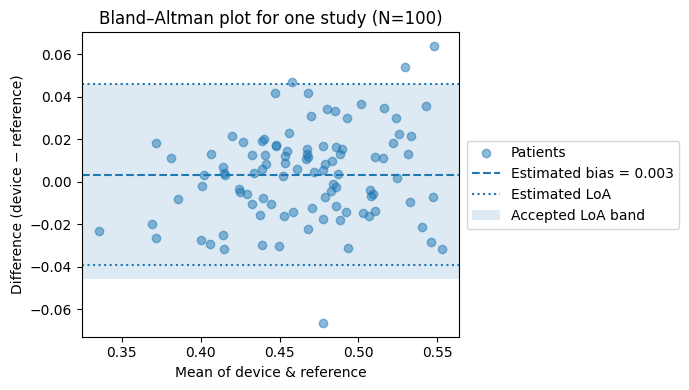
Worked example (CTR) : If μ = 0.46, then LoA band is $\pm 0.046$ and bias limit is $\pm 0.009$.
'''
Set the Acceptance Criteria

#  Rule of thumb for Bland–Altman on continuous outputs:
#   LoA ≈ ±10% of mean physiological value
#   Bias ≈ ±2% of mean physiological value
'''

loa_fraction = 0.10   # 10% of mean
bias_fraction = 0.02  # 2% of mean

loa_half_width = loa_fraction * mean_true_ctr
bias_limit = bias_fraction * mean_true_ctr

loa_lower_accept = -loa_half_width
loa_upper_accept =  loa_half_width

print(f"Accepted LoA: [{loa_lower_accept:.3f}, {loa_upper_accept:.3f}]")
print(f"Accepted bias magnitude: ±{bias_limit:.3f}")
Output :
Accepted LoA: [-0.046, 0.046]
Accepted bias magnitude: ±0.009
Step 4 : Define “pass” using bootstrap confidence intervals 🔗
In each simulated study (with sample size $N$), we need an objective rule to judge whether it meets the Bland Altman criteria or not, in an uncertain environment. Using point estimates alone (one bias value and one value of LoA) can look “good” or “bad” by chance alone, especially if $N$ is small. So, we have to use bootstrap confidence intervals (CIs).
Begin with paired data, Take :
\[(x_i, y_i),\quad i = 1,\ldots,N\]and compute differences
\[d_i = y_i - x_i\]Calculate the Bland Altman statistics for the study :
- $\text{bias} = \frac{1}{N}\sum_{i=1}^{N} (y_i - x_i) = \bar{d}$
- Limits of Agreement (LoA) :
\(\text{LoA}_{\text{lower}} = \bar{d} - 1.96\, s_d, \qquad\text{LoA}_{\text{upper}} = \bar{d} + 1.96\, s_d\)
Now estimate uncertainty with bootstrap :
- Loop $B$ times (eg, $ B = 1000$) : resample $N$ patients with replacement (either resample the pairs $(x_i, y_i)$ or resample the differences $d_i$).
- Recalculate bias, LoA (both lower and upper) for each resample
- Use the 2.5th and 97.5th percentile across the $B$ resamples to form 95% CIs for bias, LoA_lower and LoA_upper.
Pass rule : the study passes only if the whole confidence interval is within the permissible limits :
- Bias CI is within the allowed bias range
\(\mathrm{CI}_{95\%}(\text{bias}) \subseteq [-\text{bias\_limit},\ +\text{bias\_limit}]\) - LoA_lower CI does not go below its allowed lower boundary
\(\mathrm{CI}_{95\%}(\mathrm{LoA}_{\mathrm{lower}}) \ge \text{loa\_lower\_accept}\) - LoA_upper does not exceed the allowable upper boundary
\(\mathrm{CI}_{95\%}(\mathrm{LoA}_{\mathrm{upper}}) \le \text{loa\_upper\_accept}\)
This results in a single “True/False pass” for the simulated study that we will count in large numbers in next step.
'''
Bland–Altman analysis for one simulated study
'''
def bland_altman_with_bootstrap(true_vals, device_vals, n_boot=1000):
    """
    Compute Bland–Altman bias, LoA, and bootstrap 95% CIs.
    """
    diff = device_vals - true_vals
    means = (device_vals + true_vals) / 2.0

    bias = diff.mean()
    sd = diff.std(ddof=1)
    loa_lower = bias - 1.96 * sd
    loa_upper = bias + 1.96 * sd

    # Bootstrap the differences
    n = len(diff)
    boot_bias = np.empty(n_boot)
    boot_loa_lower = np.empty(n_boot)
    boot_loa_upper = np.empty(n_boot)

    for b in range(n_boot):
        sample = np.random.choice(diff, size=n, replace=True)
        b_bias = sample.mean()
        b_sd = sample.std(ddof=1)
        boot_bias[b] = b_bias
        boot_loa_lower[b] = b_bias - 1.96 * b_sd
        boot_loa_upper[b] = b_bias + 1.96 * b_sd

    bias_ci = np.percentile(boot_bias, [2.5, 97.5])
    loa_lower_ci = np.percentile(boot_loa_lower, [2.5, 97.5])
    loa_upper_ci = np.percentile(boot_loa_upper, [2.5, 97.5])

    return {
        "means": means,
        "diff": diff,
        "bias": bias,
        "bias_ci": bias_ci,
        "loa_lower": loa_lower,
        "loa_upper": loa_upper,
        "loa_lower_ci": loa_lower_ci,
        "loa_upper_ci": loa_upper_ci,
    }

# Lets simulate ONE study with N = 100 patients
n_study = 100
true_study = np.random.normal(mean_true_ctr, std_true_ctr, size=n_study)
device_study = simulate_device_measurements(true_study, device_bias, device_sd)
metrics_example = bland_altman_with_bootstrap(true_study, device_study)

# Plot the Bland–Altman figure for this one study
fig, ax = plt.subplots(figsize=(7, 4))

# Leave extra space on the right for the legend
fig.subplots_adjust(right=0.7)

ax.scatter(metrics_example["means"], metrics_example["diff"],
           alpha=0.5, label="Patients")

ax.axhline(metrics_example["bias"], linestyle="--",
           label=f"Estimated bias = {metrics_example['bias']:.3f}")
ax.axhline(metrics_example["loa_lower"], linestyle=":",
           label="Estimated LoA")
ax.axhline(metrics_example["loa_upper"], linestyle=":")

# Acceptance band
ax.axhspan(loa_lower_accept, loa_upper_accept, alpha=0.15,
           label="Accepted LoA band")

ax.set_xlabel("Mean of device & reference")
ax.set_ylabel("Difference (device − reference)")
ax.set_title(f"Bland–Altman plot for one study (N={n_study})")

# Legend on the right, outside the axes
ax.legend(loc="center left", bbox_to_anchor=(1.02, 0.5), borderaxespad=0.)

plt.tight_layout()
plt.show()
# Decide when a study "passes" the acceptance criteria

def study_passes(metrics, bias_limit, loa_lower_accept, loa_upper_accept):
    """
    Return True if this study passes:
    - bias CI inside [-bias_limit, +bias_limit]
    - LoA CIs inside [loa_lower_accept, loa_upper_accept]
    """
    bias_ci = metrics["bias_ci"]
    loa_lower_ci = metrics["loa_lower_ci"]
    loa_upper_ci = metrics["loa_upper_ci"]

    bias_ok = (bias_ci[0] >= -bias_limit) and (bias_ci[1] <= bias_limit)
    lower_ok = (loa_lower_ci[0] >= loa_lower_accept)
    upper_ok = (loa_upper_ci[1] <= loa_upper_accept)

    return bias_ok and lower_ok and upper_ok

# Quick test on our example study
print("Example study passes?",
      study_passes(metrics_example, bias_limit, loa_lower_accept, loa_upper_accept))
Output :
Example study passes? False
'''
Under these assumptions, a single simulated N=100 study failed
the CI based acceptance rule, and the estimated power at N=100 is ~0.40
in the sweep below
'''
Step 5 : Estimate power across N, then choose N 🔗
At this point, Step 4 gives you a pass/fail result for one simulated study of size $N$. Step 5 turns that into what matters for us : power, that is :
\[\mathrm{Power}(N) = \mathbb{P}\!\left(\text{a study of size } N \text{ passes the acceptance criteria}\right)\]As there is no clean analytic solution with bootstrap confidence intervals, a Monte Carlo estimate of Power ($N$) is to run many virtual experiments and count how often they pass. To be specific, for a candidate sample size N :
- Repeat
n_simulationstimes (eg , 1000):- $N $ ground truth values are selected using the population model (Step 1)
- Produce $N$ device values using the error model (Step 2)
- Compute Bland Altman bias/LoA with bootstrapped confidence intervals (Step 4)
- Apply the pass rule to return True/False
- Estimated power is :
\(\mathrm{Power}(N) = \frac{\text{number of passes}}{n_{\text{simulations}}}\)
This is exactly what our estimate_power_for_n function is doing , with the sweep through sample_sizes determining the table of $N$ vs power.
# For a given N, simulate many studies and estimate power

def estimate_power_for_n(n, n_simulations=1000, n_bootstrap=1000):
    """
    Generate 'n_simulations' virtual studies of size n,
    and return the fraction that pass = estimated power.
    """
    passes = 0
    for _ in range(n_simulations):
        true_vals = np.random.normal(mean_true_ctr, std_true_ctr, size=n)
        device_vals = simulate_device_measurements(true_vals, device_bias, device_sd)
        metrics = bland_altman_with_bootstrap(true_vals, device_vals, n_boot=n_bootstrap)
        if study_passes(metrics, bias_limit, loa_lower_accept, loa_upper_accept):
            passes += 1
    return passes / n_simulations

# Sweep a grid of sample sizes (patients)
sample_sizes = [20, 30, 40, 50, 60, 80, 100, 120, 150, 200, 400, 800, 1000]

rows = []
for n in sample_sizes:
    power = estimate_power_for_n(n, n_simulations=1000, n_bootstrap=500)
    rows.append({"sample_size": n, "power": power})

power_df = pd.DataFrame(rows)

# Table of sample size vs estimated power
print("\nSample size vs estimated power:\n")
print(power_df.to_string(index=False))

# Power curve plot
target_power = 0.80

plt.figure()
plt.plot(power_df["sample_size"], power_df["power"], marker="o")
plt.axhline(target_power, linestyle="--",
            label=f"Target power = {target_power:.0%}")
plt.xlabel("Sample size N")
plt.ylabel("Estimated power")
plt.title("Probability that the Bland–Altman study will pass")
plt.legend()
plt.tight_layout()
Sample size vs estimated power:

 sample_size  power
          20  0.089
          30  0.146
          40  0.195
          50  0.226
          60  0.241
          80  0.314
         100  0.375
         120  0.468
         150  0.505
         200  0.656
         400  0.914
         800  0.998
        1000  0.999
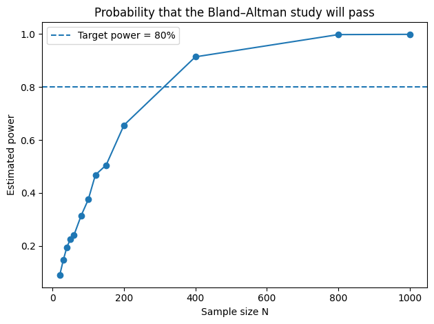
Now that you have Power(N), select a power goal (typically 80% or 90%), then select the smallest N that equals or exceeds it. Looking back at the example solution output, power goes from about $0.64$ for $N = 200$ to about $0.93$ for $N = 400,$ so the smallest $N$ for 80% is $N = 400$.
Results and Takeaways 🔗
The walkthrough above showed how the simulation is run for a single scenario (the CTR example). In practice, you will need to look up required sample sizes for different expected device error levels without having to repeat the entire simulation. This section provides tables and plots that connect the size of the device error directly with the minimum $N$ required for 80% and 90% power.
To make the tables generally applicable, we normalize the problem : ground truth is normally distributed with parameters $\mathcal{N}(0,1)$, and the LoA acceptance criterion is $\pm 0.2$. If you want to apply this to a real device, you scale your expected error standard deviation by the ratio of your LoA target to 0.2 (see “How to use these tables” at the end of this section).
We sweep three error models :
- Additive only : the difference $d=y−x$ is drawn from $\mathcal{N}(0,σ_{add})$, with $σ_{add}$ ranging from 0.001 to 0.100 in 50 steps.
- Proportional only : the difference is drawn from $\mathcal{N}(0,σ_{prop}\cdot \lvert x \rvert)$, with $σ_{prop}$ ranging from 0% to 10% in steps of 0.5%.
- Combined : the difference is drawn from $\mathcal{N}(0,σ_{add}+σ_{prop}\cdot \lvert x \rvert)$, sweeping both axes simultaneously in a 50 × 20 grid.
For each cell in the grid, we perform 300 simulated studies, each with 300 bootstrap resamples. A study “passes” when the bootstrap 95% CIs for both the upper and lower LoA fall entirely inside $[-0.2, +0.2]$. Power is the fraction of simulated studies that pass, and we report the smallest $N$ from the grid that first reaches the target power.
Simulation setup 🔗
The code below is the same as the walkthrough (Steps 1 through 5) but we put everything in functions so we can sweep over parameter grids. We set a random seed so we can reproduce the results like we did before, and we work on a normalized scale ground truth $\sim \mathcal{N}(0, 1)$, LoA acceptance band $\pm 0.2$.
'''
Imports and constants for the precomputed tables.
Ground truth is standard normal, LoA target is ±0.2.
'''
import os
import numpy as np
import pandas as pd
import matplotlib.pyplot as plt
from matplotlib.colors import LogNorm


SEED = 12345
RNG = np.random.default_rng(SEED)

MEAN_TRUE = 0.0
SD_TRUE = 1.0

LOA_HALF_WIDTH = 0.2
Z_VALUE = 1.96

N_SIMULATIONS = 300
N_BOOTSTRAP = 300

''' Candidate sample sizes to sweep '''
N_GRID = [
    10, 15, 20, 25, 30, 40, 50, 60, 80, 100,
    120, 150, 200, 250, 300, 400, 600, 800, 1000,
    1500, 2000, 3000, 5000, 8000, 10000,
]

MAX_TARGET_POWER = 0.9

OUTPUT_DIR = "results_takeaways_output"

''' We cache bootstrap index arrays so every call with the same
(n, n_boot) reuses the same random draw '''
BOOTSTRAP_INDICES_CACHE = {}

def get_bootstrap_indices(n, n_boot, rng):
    key = (n, n_boot)
    if key not in BOOTSTRAP_INDICES_CACHE:
        BOOTSTRAP_INDICES_CACHE[key] = rng.integers(0, n, size=(n_boot, n))
    return BOOTSTRAP_INDICES_CACHE[key]
In Step 2, we modeled the device as $ y_i = x_i + b + \varepsilon_i$. For sweep tables we work directly with difference $d_i = y_i - x_i$ and allow the error SD to depend on the measurement magnitude. The function below handles all three cases in one call : pure additive ($σ_{prop} = 0$), pure proportional ($σ_{add} = 0$), or combined.
def simulate_differences(n, sd_add, sd_prop, rng):
    '''Draw n paired differences under the additive + proportional model.
    If sd_prop is zero we skip the ground-truth draw entirely.'''
    if sd_prop == 0.0:
        return rng.normal(0.0, sd_add, size=n)

    x = rng.normal(MEAN_TRUE, SD_TRUE, size=n)
    sd = sd_add + sd_prop * np.abs(x)
    return rng.normal(0.0, sd, size=n)
The bootstrap pass rule is the same as Step 4, but adapted for batch sweeping. We bootstrap the differences, calculate the 95% CIs for both limits of the LoA, and check whether the full CI is within $[−0.2,+0.2]$.
def loa_ci_from_diff(diff, n_boot, rng):
    '''Bootstrap the 95% CIs for lower and upper LoA.'''
    n = diff.size
    indices = get_bootstrap_indices(n, n_boot, rng)
    samples = diff[indices]
    means = samples.mean(axis=1)
    sds = samples.std(axis=1, ddof=1)

    loa_lower = means - Z_VALUE * sds
    loa_upper = means + Z_VALUE * sds

    loa_lower_ci = np.percentile(loa_lower, [2.5, 97.5])
    loa_upper_ci = np.percentile(loa_upper, [2.5, 97.5])

    return loa_lower_ci, loa_upper_ci


def study_passes(diff, loa_half_width, n_boot, rng):
    '''Return True when the full bootstrap CI for both LoA limits
    falls inside [-loa_half_width, +loa_half_width].'''
    loa_lower_ci, loa_upper_ci = loa_ci_from_diff(diff, n_boot, rng)
    lower_ok = loa_lower_ci[0] >= -loa_half_width
    upper_ok = loa_upper_ci[1] <= loa_half_width
    return lower_ok and upper_ok
Now we wrap power estimation as we did in the Step 5 : for a candidate $N$, we perform many virtual studies, count how many pass and report the fraction. power_curve_for_params tries many candidates on the grid and stops early if we reach the target power. first_n_for target looks up the first $N$ that reaches a given threshold.
def estimate_power_for_n(n, sd_add, sd_prop, loa_half_width, n_sim, n_boot, rng):
    '''Monte Carlo power : fraction of n_sim virtual studies that pass.'''
    passes = 0
    for _ in range(n_sim):
        diff = simulate_differences(n, sd_add, sd_prop, rng)
        if study_passes(diff, loa_half_width, n_boot, rng):
            passes += 1
    return passes / n_sim


def power_curve_for_params(sd_add, sd_prop, n_grid, loa_half_width, n_sim, n_boot, rng):
    '''Sweep candidate sample sizes and return (ns, powers).
    Stops early once MAX_TARGET_POWER is reached.'''
    ns, powers = [], []
    for n in n_grid:
        power = estimate_power_for_n(
            n, sd_add, sd_prop, loa_half_width, n_sim, n_boot, rng
        )
        ns.append(n)
        powers.append(power)
        if power >= MAX_TARGET_POWER:
            break
    powers = np.maximum.accumulate(powers)
    return np.array(ns), np.array(powers)


def first_n_for_target(ns, powers, target_power):
    '''Return the first N whose power >= target, or NaN if none qualifies.'''
    for n, power in zip(ns, powers):
        if power >= target_power:
            return n, power
    if len(powers) == 0:
        return np.nan, np.nan
    return np.nan, powers[-1]
We also define two small helpers for saving line plots and heatmaps so the sweep code stays clean.
def save_line_plot(x, y, xlabel, ylabel, title, output_path):
    plt.figure(figsize=(10, 6))
    plt.plot(x, y, marker="o", linewidth=2, markersize=4)
    plt.xlabel(xlabel)
    plt.ylabel(ylabel)
    plt.title(title)
    plt.grid(True, alpha=0.3)

    # Add reference lines for key sample sizes
    reference_ns = [100, 250, 500, 1000, 5000, 10000]
    for ref_n in reference_ns:
        if ref_n <= plt.ylim()[1]:
            plt.axhline(y=ref_n, color='gray', linestyle='--', alpha=0.4, linewidth=0.8)
            if ref_n == 250:
                plt.text(plt.xlim()[1] * 0.98, ref_n, f'N={ref_n}',
                        verticalalignment='bottom', horizontalalignment='right',
                        fontsize=9, color='red', fontweight='bold')
            elif ref_n in [100, 500, 1000]:
                plt.text(plt.xlim()[1] * 0.98, ref_n, f'N={ref_n}',
                        verticalalignment='bottom', horizontalalignment='right',
                        fontsize=8, color='gray')

    plt.tight_layout()
    plt.savefig(output_path, dpi=200)
    plt.close()

def save_heatmap(df, title, output_path, x_label, y_label, x_formatter, y_formatter):
    data = df.astype(float).values
    fig, ax = plt.subplots(figsize=(12, 9))

    vmin = np.nanmin(data)
    vmax = np.nanmax(data)

    if vmax / vmin > 100:
        im = ax.imshow(data, origin="lower", aspect="auto", cmap="viridis",
                      norm=LogNorm(vmin=max(vmin, 1), vmax=vmax))
    else:
        im = ax.imshow(data, origin="lower", aspect="auto", cmap="viridis")

    # Add contour lines at key sample sizes
    X, Y = np.meshgrid(np.arange(len(df.columns)), np.arange(len(df.index)))
    contour_levels = [50, 100, 150, 250, 500, 1000, 1500, 3000]
    contours = ax.contour(X, Y, data, levels=contour_levels,
                         colors='white', linewidths=1.5, alpha=0.6)
    ax.clabel(contours, inline=True, fontsize=9, fmt='N=%d')

    ax.set_xticks(np.arange(len(df.columns)))
    ax.set_yticks(np.arange(len(df.index)))
    ax.set_xticklabels([x_formatter(x) for x in df.columns], rotation=45, ha="right")
    ax.set_yticklabels([y_formatter(y) for y in df.index])
    ax.set_xlabel(x_label)
    ax.set_ylabel(y_label)
    ax.set_title(title)
    fig.colorbar(im, ax=ax, label="Required sample size")
    plt.tight_layout()
    plt.savefig(output_path, dpi=200)
    plt.close()
Additive error model results 🔗
We sweep $\sigma_{add}$ from 0.001 to 0.020 in 50 equally spaced steps, with $\sigma_{prop}$ = 0 (no proportional component). For each value we compute the full power curve across N_GRID , then look up the first $N$ that reaches 80% and 90% power.
additive_sds = np.round(np.linspace(0.001, 0.100, 50), 3)

additive_rows = []
for sd_add in additive_sds:
    ns, powers = power_curve_for_params(
        sd_add, 0.0, N_GRID, LOA_HALF_WIDTH, N_SIMULATIONS, N_BOOTSTRAP, RNG
    )
    n_08, p_08 = first_n_for_target(ns, powers, 0.8)
    n_09, p_09 = first_n_for_target(ns, powers, 0.9)
    additive_rows.append({
        "additive_sd": sd_add,
        "n_for_power_0_8": n_08, "power_at_n_0_8": p_08,
        "n_for_power_0_9": n_09, "power_at_n_0_9": p_09,
    })

additive_df = pd.DataFrame(additive_rows)
additive_df.to_csv(os.path.join(OUTPUT_DIR, "additive_required_n.csv"), index=False)

''' Line plots for both power targets '''
save_line_plot(
    additive_df["additive_sd"], additive_df["n_for_power_0_8"],
    "Additive error SD", "Required sample size (power >= 0.8)",
    "Additive error model: required N for 0.8 power",
    os.path.join(OUTPUT_DIR, "additive_required_n_power_0_8.png"),
)
save_line_plot(
    additive_df["additive_sd"], additive_df["n_for_power_0_9"],
    "Additive error SD", "Required sample size (power >= 0.9)",
    "Additive error model: required N for 0.9 power",
    os.path.join(OUTPUT_DIR, "additive_required_n_power_0_9.png"),
)
| Additive SD | N for 0.8 power | Power at N | N for 0.9 power | Power at N |
|---|---|---|---|---|
| 0.001 | 10 | 1.00 | 10 | 1.00 |
| 0.003 | 10 | 1.00 | 10 | 1.00 |
| 0.005 | 10 | 1.00 | 10 | 1.00 |
| 0.007 | 10 | 1.00 | 10 | 1.00 |
| 0.009 | 10 | 1.00 | 10 | 1.00 |
| 0.011 | 10 | 1.00 | 10 | 1.00 |
| 0.013 | 10 | 1.00 | 10 | 1.00 |
| 0.015 | 10 | 1.00 | 10 | 1.00 |
| 0.017 | 10 | 1.00 | 10 | 1.00 |
| 0.019 | 10 | 1.00 | 10 | 1.00 |
| 0.021 | 10 | 1.00 | 10 | 1.00 |
| 0.023 | 10 | 1.00 | 10 | 1.00 |
| 0.025 | 10 | 1.00 | 10 | 1.00 |
| 0.027 | 10 | 1.00 | 10 | 1.00 |
| 0.029 | 10 | 1.00 | 10 | 1.00 |
| 0.031 | 10 | 1.00 | 10 | 1.00 |
| 0.033 | 10 | 1.00 | 10 | 1.00 |
| 0.035 | 10 | 1.00 | 10 | 1.00 |
| 0.037 | 10 | 1.00 | 10 | 1.00 |
| 0.039 | 10 | 1.00 | 10 | 1.00 |
| 0.041 | 10 | 1.00 | 10 | 1.00 |
| 0.043 | 10 | 0.98 | 10 | 0.98 |
| 0.045 | 10 | 0.97 | 10 | 0.97 |
| 0.047 | 10 | 0.99 | 10 | 0.99 |
| 0.049 | 10 | 0.95 | 10 | 0.95 |
| 0.052 | 10 | 0.90 | 10 | 0.90 |
| 0.054 | 10 | 0.87 | 15 | 0.93 |
| 0.056 | 10 | 0.82 | 15 | 0.94 |
| 0.058 | 10 | 0.87 | 20 | 0.93 |
| 0.060 | 15 | 0.85 | 20 | 0.91 |
| 0.062 | 20 | 0.85 | 25 | 0.92 |
| 0.064 | 20 | 0.82 | 25 | 0.90 |
| 0.066 | 25 | 0.81 | 40 | 0.93 |
| 0.068 | 30 | 0.80 | 40 | 0.92 |
| 0.070 | 40 | 0.87 | 50 | 0.90 |
| 0.072 | 50 | 0.87 | 60 | 0.91 |
| 0.074 | 50 | 0.81 | 80 | 0.91 |
| 0.076 | 80 | 0.86 | 100 | 0.94 |
| 0.078 | 100 | 0.91 | 100 | 0.91 |
| 0.080 | 120 | 0.86 | 150 | 0.95 |
| 0.082 | 150 | 0.84 | 200 | 0.93 |
| 0.084 | 150 | 0.80 | 250 | 0.95 |
| 0.086 | 250 | 0.82 | 300 | 0.92 |
| 0.088 | 400 | 0.88 | 600 | 0.98 |
| 0.090 | 600 | 0.93 | 600 | 0.93 |
| 0.092 | 800 | 0.90 | 800 | 0.90 |
| 0.094 | 1500 | 0.93 | 1500 | 0.93 |
| 0.096 | 3000 | 0.95 | 3000 | 0.95 |
| 0.098 | 5000 | 0.85 | 8000 | 0.98 |
| 0.100 | — | 0.45 | — | 0.45 |
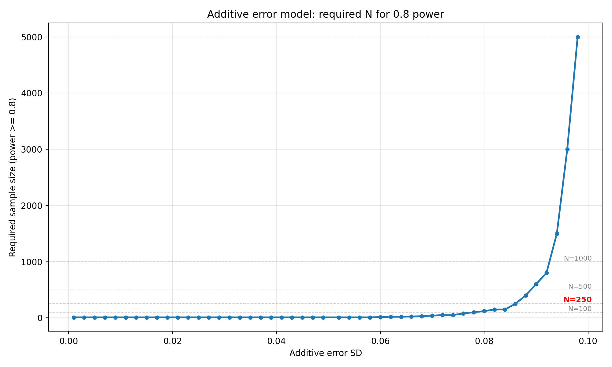
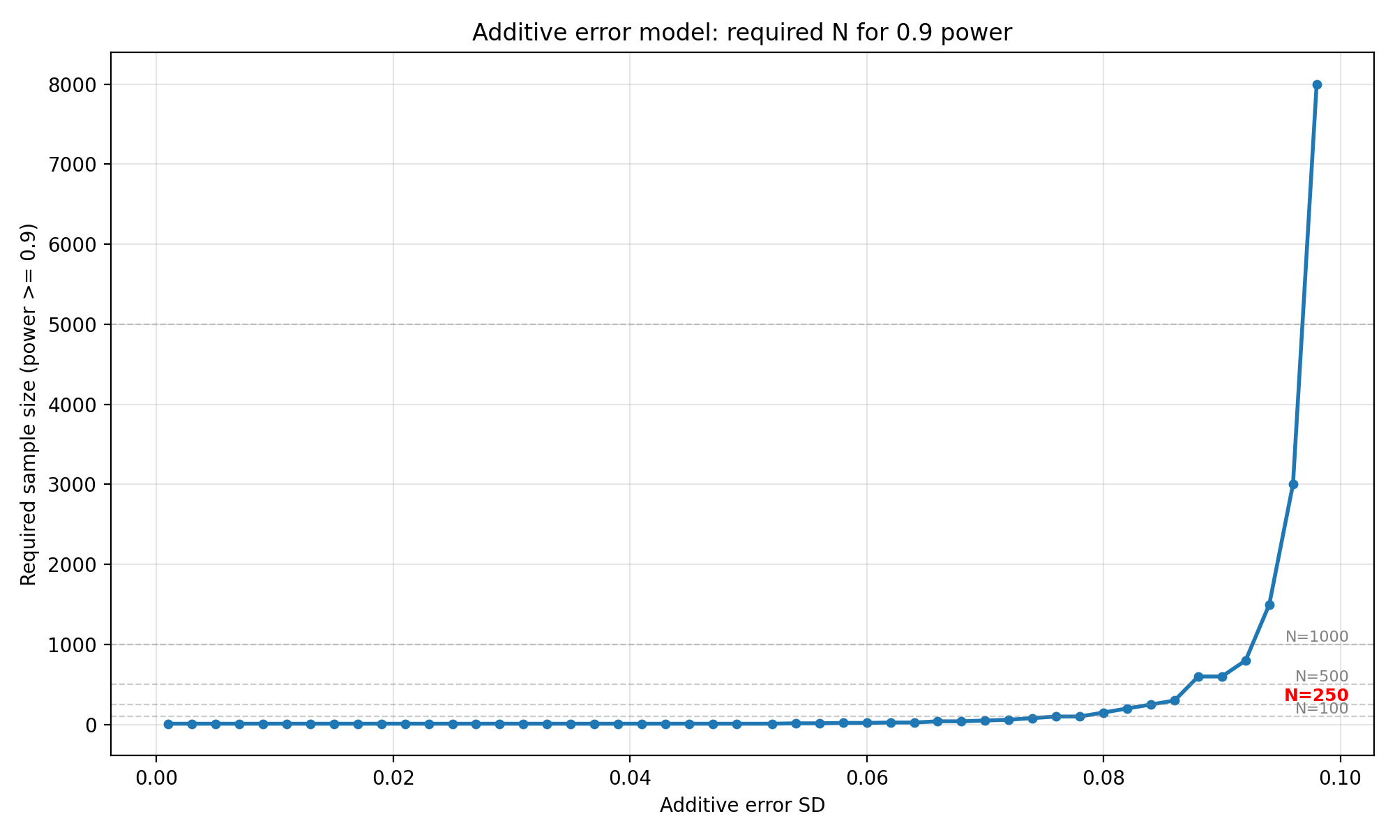
Interpretation : When the error is purely additive, for SDs up to 0.052, $N = 10$ is sufficient at both 80% and 90% power. Beyond $\sigma_{\text{add}} \approx 0.052$, the required $N$ begins to climb steeply, $N = 20$ at 0.062, $N = 150 $ at 0.084 , $N = 250$ at 0.086 (for 0.8 power), reaching $N = 5000$ at 0.098. For $N = 250$, the additive SD must stay below roughly 0.086 to have 80% power with 250 patients. At $\sigma_{\text{add}} = 0.100$ (half the LoA half-width), even $N = 10,000$ is insufficient as the simulation never reaches 80% power.
Proportional error model results 🔗
We sweep $\sigma_{prop}$ from 0% to 10% of $\lvert x \rvert$ in steps of 0.5%, with $\sigma_{add} = 0$ (no additive component). Because the ground truth has unit variance, proportional error of $k$% means the effective SD for a patient with $\lvert x \rvert = 1$ is $0.01k$.
proportional_sds = np.round(np.arange(0.0, 0.100 + 1e-9, 0.0025), 4)

proportional_rows = []
for sd_prop in proportional_sds:
    ns, powers = power_curve_for_params(
        0.0, sd_prop, N_GRID, LOA_HALF_WIDTH, N_SIMULATIONS, N_BOOTSTRAP, RNG
    )
    n_08, p_08 = first_n_for_target(ns, powers, 0.8)
    n_09, p_09 = first_n_for_target(ns, powers, 0.9)
    proportional_rows.append({
        "proportional_sd": sd_prop,
        "n_for_power_0_8": n_08, "power_at_n_0_8": p_08,
        "n_for_power_0_9": n_09, "power_at_n_0_9": p_09,
    })

proportional_df = pd.DataFrame(proportional_rows)
proportional_df.to_csv(os.path.join(OUTPUT_DIR, "proportional_required_n.csv"), index=False)

save_line_plot(
    proportional_df["proportional_sd"] * 100.0, proportional_df["n_for_power_0_8"],
    "Proportional error SD (% of |x|)", "Required sample size (power >= 0.8)",
    "Proportional error model: required N for 0.8 power",
    os.path.join(OUTPUT_DIR, "proportional_required_n_power_0_8.png"),
)
save_line_plot(
    proportional_df["proportional_sd"] * 100.0, proportional_df["n_for_power_0_9"],
    "Proportional error SD (% of |x|)", "Required sample size (power >= 0.9)",
    "Proportional error model: required N for 0.9 power",
    os.path.join(OUTPUT_DIR, "proportional_required_n_power_0_9.png"),
)
| Proportional SD (%) | N for 0.8 power | Power at N | N for 0.9 power | Power at N |
|---|---|---|---|---|
| 0.0 | 10 | 1.00 | 10 | 1.00 |
| 0.5 | 10 | 1.00 | 10 | 1.00 |
| 1.0 | 10 | 1.00 | 10 | 1.00 |
| 1.5 | 10 | 1.00 | 10 | 1.00 |
| 2.0 | 10 | 1.00 | 10 | 1.00 |
| 2.5 | 10 | 1.00 | 10 | 1.00 |
| 3.0 | 10 | 0.98 | 10 | 0.98 |
| 3.5 | 10 | 0.96 | 10 | 0.96 |
| 4.0 | 10 | 0.91 | 10 | 0.91 |
| 4.5 | 10 | 0.84 | 15 | 0.90 |
| 5.0 | 15 | 0.87 | 40 | 0.96 |
| 5.5 | 20 | 0.82 | 40 | 0.93 |
| 6.0 | 40 | 0.83 | 80 | 0.94 |
| 6.5 | 80 | 0.83 | 100 | 0.93 |
| 7.0 | 120 | 0.84 | 150 | 0.90 |
| 7.5 | 200 | 0.84 | 250 | 0.91 |
| 8.0 | 300 | 0.81 | 400 | 0.92 |
| 8.5 | 800 | 0.92 | 800 | 0.92 |
| 9.0 | 1500 | 0.85 | 2000 | 0.94 |
| 9.5 | 5000 | 0.89 | 8000 | 0.99 |
| 10.0 | — | 0.27 | — | 0.27 |
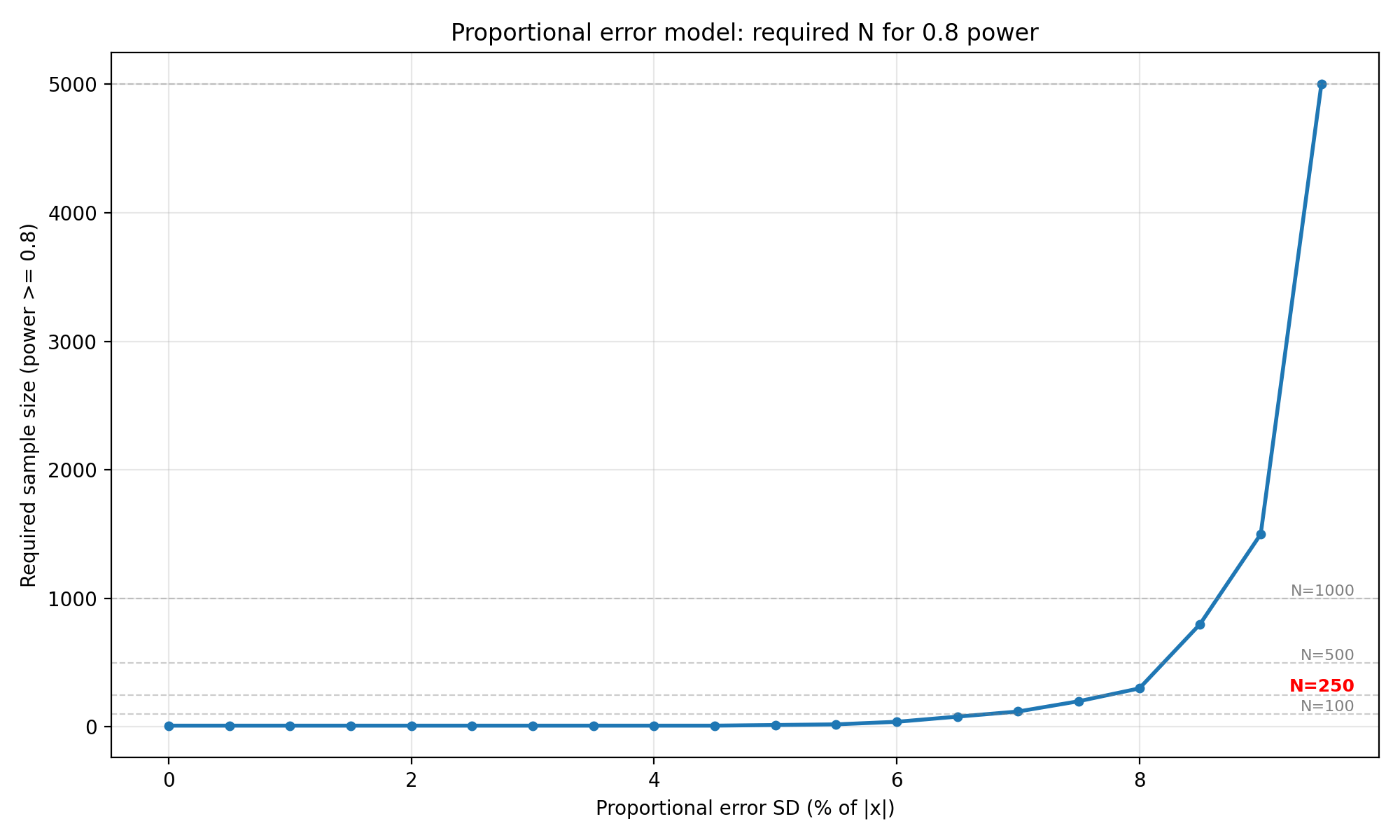
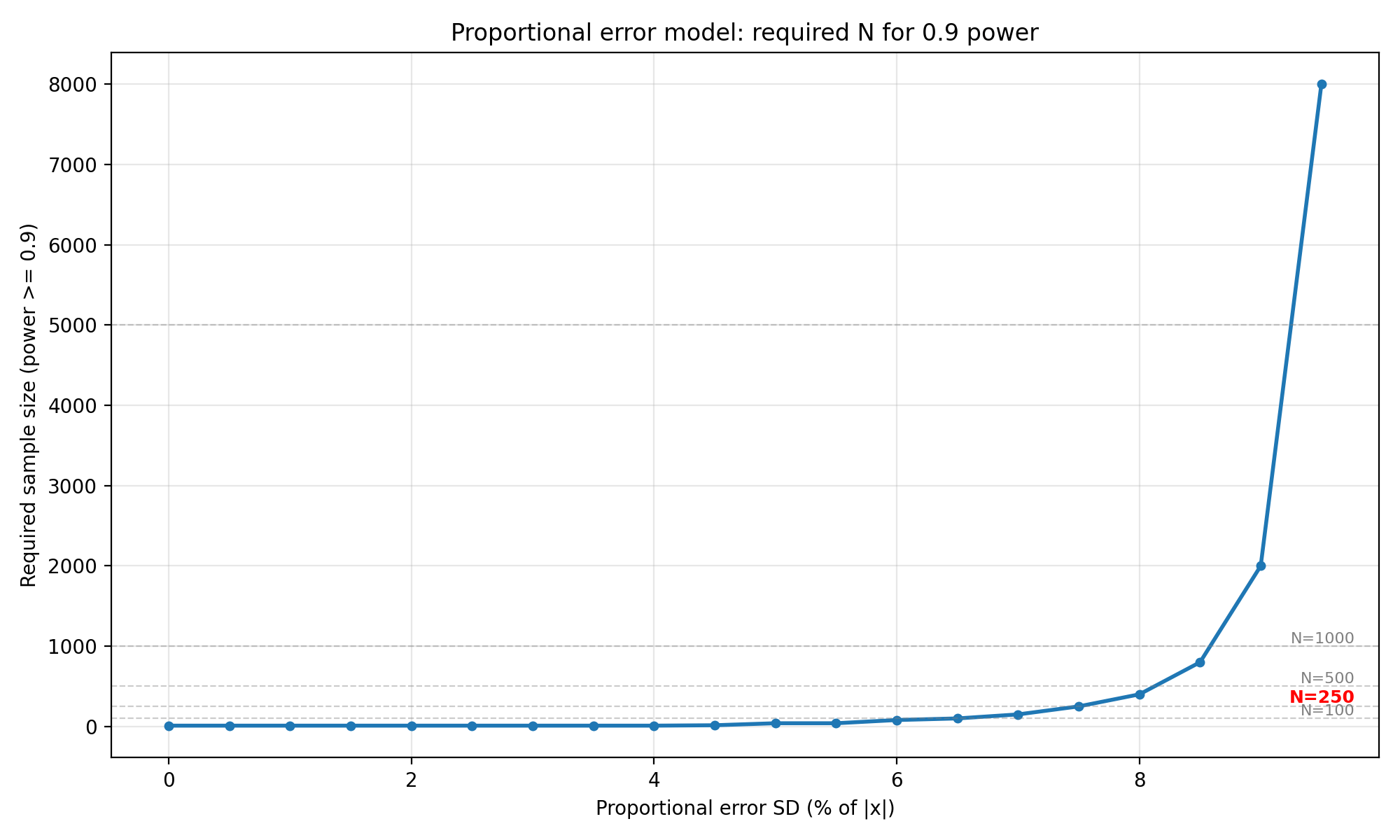
Interpretation : The proportional error model stays flat at $N = 10$ until $\sigma_{prop}$ reaches about 4.5% of $\lvert x \rvert$. Beyond that, the required $N$ begins to climb,$N=15$ at 5.0%, $N=200$ at 7.5%, $N = 800$ at 8.5%, and $N=5000 $ at 9.5% (all for 0.8 power). For the 0.9 power target the curve shifts earlier, reaching $N=250$ at 7.5% and $N=8000$ at 9.5%. For $N=250$, proportional error must stay below roughly 7.5% to be feasible. At 10% proportional error the simulation never reaches 80% power even with $N=10,000$. This makes sense because for a standard normal ground truth, only about 32% of samples have $\lvert x \rvert > 1$, and the proportional contribution needs to be large enough relative to the LoA width (0.2) before it starts to matter.
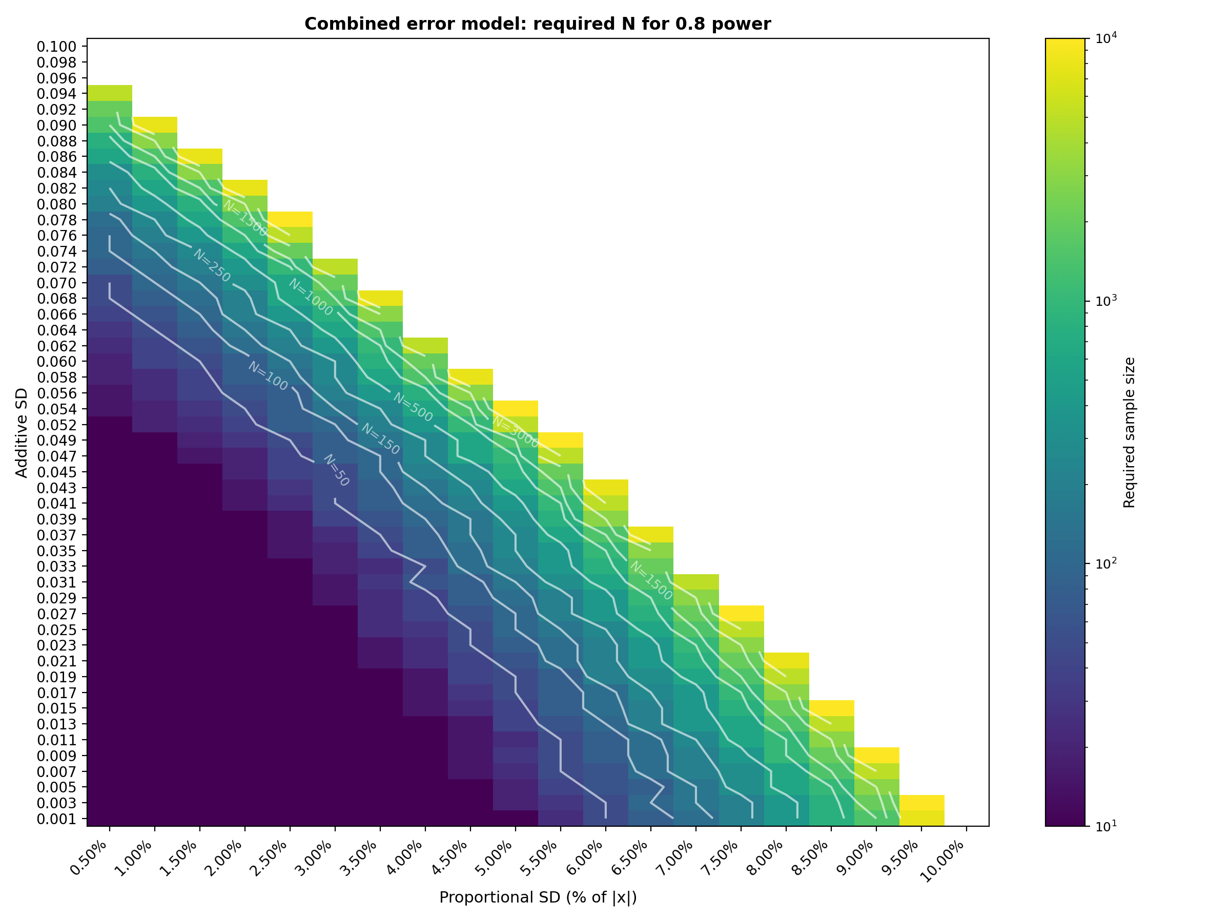
Combined error model results 🔗
We now sweep both error sources simultaneously. The total SD for each patient $\sigma_{add} + \sigma_{prop} \cdot \lvert x_i \rvert$ with $\sigma_{\text{add}} $ spanning 50 values from 0.001 to 0.100 (rows) and $\sigma_{\text{prop}}$ spanning 20 values from 0.5% to 10.0% in 0.5% steps (columns). Each cell shows the minimum $N$ from our candidate grid that reaches the target power.
The full 50 × 20 combined tables are available in the CSV files (combined_required_n_power_0_8.csv and combined_required_n_power_0_9.csv). The tables below show a representative subset (every 5th row × every other column) to keep the article readable.
proportional_sds_grid = np.round(np.arange(0.005, 0.100 + 1e-9, 0.005), 4)

combined_08 = pd.DataFrame(index=additive_sds, columns=proportional_sds_grid, dtype=float)
combined_09 = pd.DataFrame(index=additive_sds, columns=proportional_sds_grid, dtype=float)

for sd_add in additive_sds:
    for sd_prop in proportional_sds_grid:
        ns, powers = power_curve_for_params(
            sd_add, sd_prop, N_GRID, LOA_HALF_WIDTH, N_SIMULATIONS, N_BOOTSTRAP, RNG
        )
        n_08, _ = first_n_for_target(ns, powers, 0.8)
        n_09, _ = first_n_for_target(ns, powers, 0.9)
        combined_08.loc[sd_add, sd_prop] = n_08
        combined_09.loc[sd_add, sd_prop] = n_09

combined_08.to_csv(os.path.join(OUTPUT_DIR, "combined_required_n_power_0_8.csv"))
combined_09.to_csv(os.path.join(OUTPUT_DIR, "combined_required_n_power_0_9.csv"))

''' Heatmaps for both power targets '''
save_heatmap(
    combined_08, "Combined error model: required N for 0.8 power",
    os.path.join(OUTPUT_DIR, "combined_required_n_power_0_8.png"),
    "Proportional SD (% of |x|)", "Additive SD",
    lambda x: f"{x * 100:.2f}%", lambda y: f"{y:.3f}",
)
save_heatmap(
    combined_09, "Combined error model: required N for 0.9 power",
    os.path.join(OUTPUT_DIR, "combined_required_n_power_0_9.png"),
    "Proportional SD (% of |x|)", "Additive SD",
    lambda x: f"{x * 100:.2f}%", lambda y: f"{y:.3f}",
)
Required N for 0.8 power (representative subset) :
| Add \ Prop | 1.0% | 2.0% | 3.0% | 4.0% | 5.0% | 6.0% | 7.0% | 8.0% | 9.0% | 10.0% |
|---|---|---|---|---|---|---|---|---|---|---|
| 0.001 | 10 | 10 | 10 | 10 | 10 | 50 | 120 | 400 | 1500 | — |
| 0.011 | 10 | 10 | 10 | 10 | 25 | 80 | 250 | 1000 | — | — |
| 0.021 | 10 | 10 | 10 | 25 | 60 | 200 | 800 | — | — | — |
| 0.031 | 10 | 10 | 15 | 60 | 150 | 600 | 5000 | — | — | — |
| 0.041 | 10 | 15 | 50 | 120 | 400 | 5000 | — | — | — | — |
| 0.052 | 20 | 40 | 100 | 400 | 5000 | — | — | — | — | — |
| 0.062 | 40 | 120 | 400 | 5000 | — | — | — | — | — | — |
| 0.072 | 120 | 400 | 5000 | — | — | — | — | — | — | — |
| 0.082 | 600 | — | — | — | — | — | — | — | — | — |
| 0.092 | — | — | — | — | — | — | — | — | — | — |
"—" indicates the target power was not reached within the candidate grid (up to N = 10,000). Full 50 × 20 table available in combined_required_n_power_0_8.csv**.
Required N for 0.9 power (representative subset) :
| Add \ Prop | 1.0% | 2.0% | 3.0% | 4.0% | 5.0% | 6.0% | 7.0% | 8.0% | 9.0% | 10.0% |
|---|---|---|---|---|---|---|---|---|---|---|
| 0.001 | 10 | 15 | 10 | 15 | 25 | 100 | 200 | 600 | 3000 | — |
| 0.011 | 10 | 20 | 15 | 20 | 50 | 150 | 400 | 1500 | — | — |
| 0.021 | 10 | 10 | 20 | 40 | 100 | 300 | 1000 | — | — | — |
| 0.031 | 10 | 10 | 30 | 80 | 200 | 800 | 8000 | — | — | — |
| 0.041 | 15 | 20 | 60 | 150 | 600 | 5000 | — | — | — | — |
| 0.052 | 20 | 50 | 200 | 600 | 5000 | — | — | — | — | — |
| 0.062 | 60 | 150 | 600 | 5000 | — | — | — | — | — | — |
| 0.072 | 150 | 600 | 8000 | — | — | — | — | — | — | — |
| 0.082 | 600 | — | — | — | — | — | — | — | — | — |
| 0.092 | — | — | — | — | — | — | — | — | — | — |
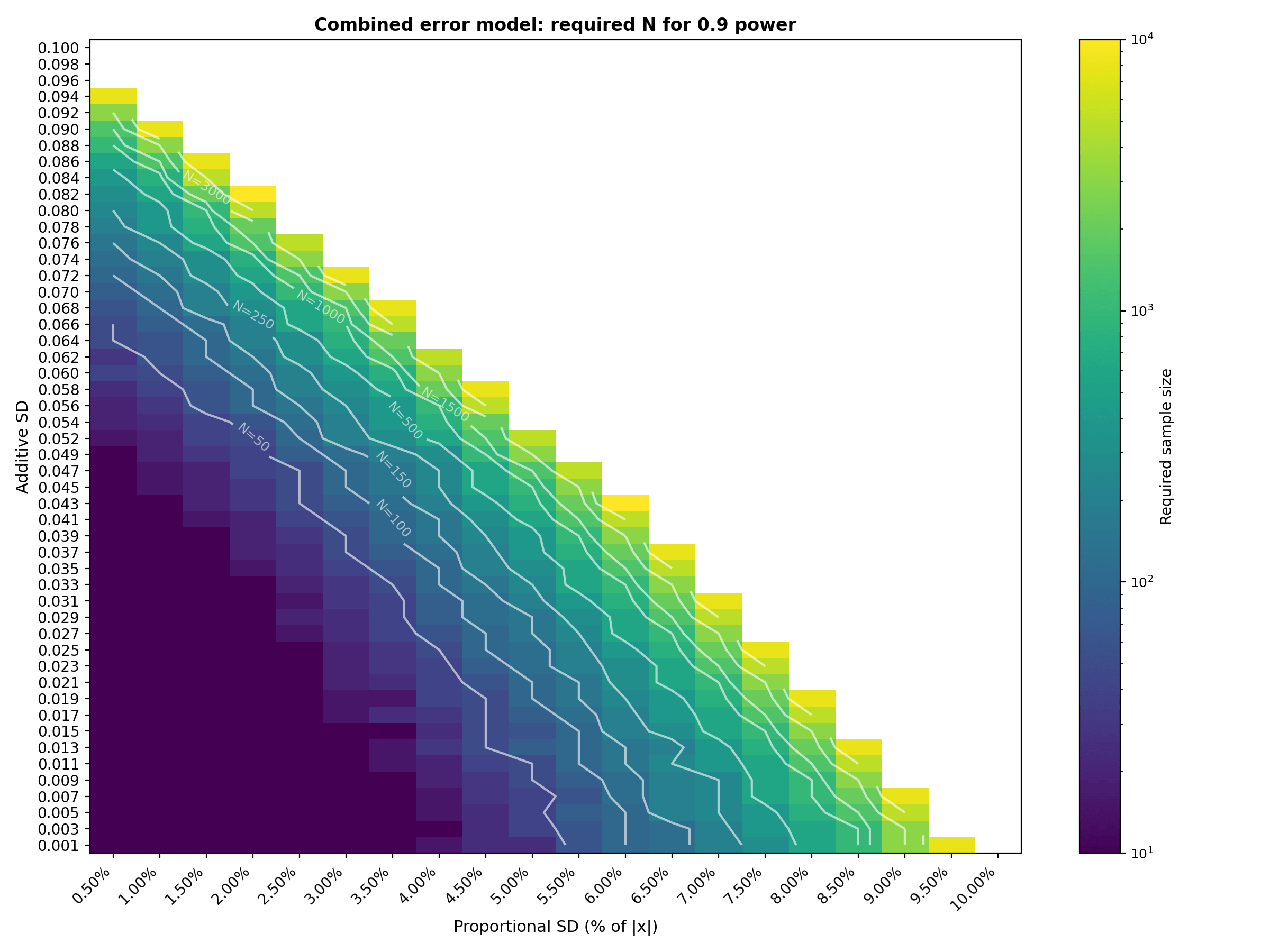
Interpretation : The combined tables show that sample size grows most aggressively in the upper right region where both additive and proportional error sources are at their highest. With the extended ranges (additive up to 0.100, proportional up to 10%, sample sizes up to 10,000), the transition from "easy" (N=10) to "infeasible" (beyond N=10,000) is now clearly visible. The N=250 contour line on the heatmaps is particularly useful as a budget constraint: it traces the boundary of error combinations that can be validated with a 250 patient study. For example, at 0.8 power, a 250 patients study is feasible along diagonal trade off where $\sigma_{add} ≤ 0.060$ with $\sigma_{prop} ≤ 3\%$, or $\sigma_{add} ≤ 0.037$ with $\sigma_{prop} ≤ 5\%$ or $\sigma_{add} ≤ 0.011$ with $\sigma_{prop} ≤ 7\%$ . Adding even a few percentage points of proportional error on top of moderate additive SD pushes the required N into the thousands. The 0.9 power table shifts this transition earlier, as expected from a stricter power requirement. The logarithmic color scale and contour lines help identify the "cliff" where required $N$ jumps by an order of magnitude over a small change in error parameters.
How to use these tables 🔗
These tables use a normalized ground truth $\mathcal{N}(0,1)$ and LoA target of $\pm0.2$. To apply them to your own device :
- Estimate your error SDs : From pilot data, literature, or engineering judgment, determine i. The constant (additive) component $\sigma^{\text{real}}_{\text{add}}$ ii. The proportional component $\sigma^{\text{real}}_{\text{prop}}$ (expressed as a fraction of $\lvert x \rvert$).
- Determine your LoA target : This is the half-width $L$ of your acceptance band in the same measurement unit as $\sigma^{\text{real}}_{\text{add}}$.
- Normalize : Calculate the normalized additive SD as $\sigma^{\text{norm}}_{\text{add}}= \sigma^{\text{real}}_{\text{add}}/(L/0.2)$. The proportional SD does not need rescaling because it is already a ratio.
- Look up the required $N$ : Find the row and column in the combined table that match your normalized additive SD and proportional SD. The cell value is the minimum sample size for the chosen power level.
- Apply a safety margin : These tables are based on 300 simulations per cell. For a production level study planning, consider re-running the simulation at higher resolution (1000+ simulations, 1000+ bootstrap resamples) around your specific operating point, and add some extra patients (say, 20% more) in case some drop out or if your assumptions don’t hold perfectly.
FAQs 🔗
Conclusion 🔗
This guide showed how to select a V&V sample size for a given definition of “pass” using Bland Altman bias and Limits of Agreement (LoA) with confidence intervals, not just point estimates. Due to the complicated forms of power expressions for bootstrapped CIs, we simulated power for a given candidate sample size $N $ by simulating numerous imaginary experiments like choosing $N $ true values from the intended use population model, generating paired devices outputs from the bias + noise error model, computing Bland Altman bias and LoA, bootstrapping to form 95% CIs for bias, LoA_lower and LoA_upper, and then using the pass rule.
This is repeated thousands of times, resulting in the number of studies that meet or exceed the power threshold. Plotting Power($N$) versus $N$ gives a decision curve and choosing a target (often 80% or 90%) and then selecting the lowest $N$ that meets or exceeds it (in the example, $N = 400$). While it is true that this is dependent on your input assumptions, so justify the population distribution, expected bias/precision and acceptance limits with literature, predicate devices and pilot data. Then run optimistic/nominal/pessimistic scenarios to quantify sensitivity and document a defensible study plan.