
The short answer 🔗
There is no single sample size for passing an area under the receiver operating characteristic curve (ROC AUC, or AUROC) of 0.90. You first need to state what pass means.
For a practical starting example, suppose the following.
- The true AUC is expected to be 0.93.
- Success requires the lower end of a two-sided 95% confidence interval to be at least 0.90.
- The test set contains equal numbers of independent condition-positive and condition-negative patients.
- You want at least an 80% chance that the completed study passes.
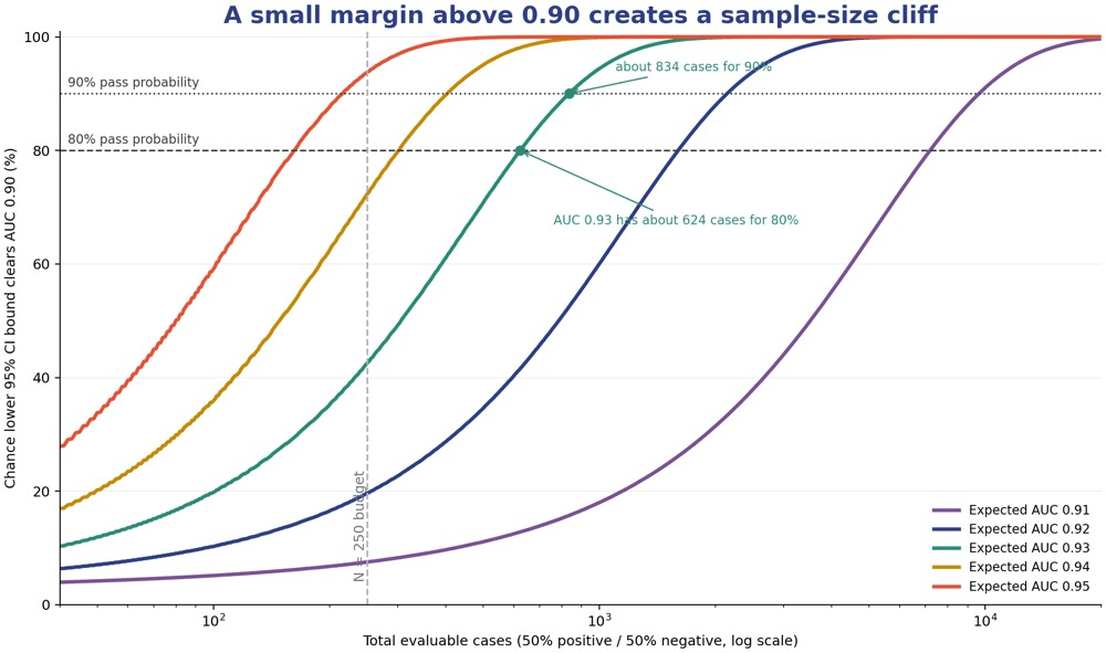
The required sample size for a Hanley and McNeil screening estimate will be approximately 624 evaluable cases, where 312 will be positive and 312 negative. When the pass probability increases to 90%, the required sample size rises to 834, where 417 will be positive and 417 negative. Accounting for 10% of non-evaluation in each stratum, the expected collection size will be 694 and 928 respectively. Continue collecting until you reach the required evaluable sample sizes.
In protocol planning, 624 will be a good starting sample size only for designing a protocol. Using the same score models, for the same design, the real numbers will be approximately 570 if a raw DeLong interval is used, 660–670 in case of a logit-DeLong interval, or 714 when a published Shu and Zou interval assurance formula is applied. First, lock the interval and then simulate the process to obtain \(N\).
| Success rule for expected AUC 0.93 | Balanced evaluable cases | What the number means |
|---|---|---|
| Point estimate \(\widehat{AUC} \ge 0.90\) | about 58 | 80% chance the point estimate clears 0.90. Uncertainty is ignored |
| Plug-in lower 95% CI evaluated at AUC 0.93 just reaches 0.90 | about 306 | only about a 50% chance of passing |
| Lower 95% CI \(\ge 0.90\) with 80% pass probability | about 624 | Hanley and McNeil screening estimate |
| Lower 95% CI \(\ge 0.90\) with 90% pass probability | about 834 | Hanley and McNeil screening estimate |
It is very important to keep in mind the main warning here. With a properly calibrated lower confidence bound, an AUC of exactly 0.90 will not give 80% or 90% assurance that the lower bound will be greater than 0.90. Under large sample calibration, the pass probability is close to 2.5% for the lower end of a two-sided 95% interval. Additional data makes the interval narrower but do not shift the truth above the acceptance threshold.
Define pass rule before choosing N 🔗
For continuous scores, AUC has a useful probability interpretation.
\[AUC=P(S^+>S^-)+\tfrac{1}{2}P(S^+=S^-),\]where \(S^+\) is a random score from positive cases and \(S^-\) is a random score from negative cases. This probability formula was originally provided by Hanley and McNeil.
The empirical AUC considers all pairs between positive and negative scores, but this does not produce \(n_+n_-\) independent pieces of information. Independent information is still coming from the cases, positive and negative patients. Ten images, lesions, or video frames from a single patient do not become ten independent cases.
There are three quantities to keep separate.
- The acceptance floor is the minimum defensible AUC, here 0.90.
- The expected true AUC is the performance you can justify from locked-algorithm pilot data, an appropriate predicate, or comparable literature.
- The pass probability is the chance that a future validation study will satisfy the complete confidence-bound rule if the expected AUC is correct.
Our exploratory automated extraction from FDA submission summaries estimated a mean observed AUC of 0.93 and a mean stated acceptance criterion of 0.89 in the reviewed examples. The linked analysis explains its spot-checking limitations. That makes 0.93 versus 0.90 a useful worked scenario. It is not a recommendation for every device.
FDA’s diagnostic-test guidance recommends reporting ROC analysis with confidence intervals. FDA’s January 2025 draft AI guidance also discusses two-sided 95% intervals and pre-specified performance goals. Device-specific guidance, special controls, intended use, clinical risk, and FDA feedback may call for another endpoint or rule.
Interactive AUC sample size calculator 🔗
Interactive planning tool
AUC lower-bound sample-size planner
Hanley and McNeil screening approximation for independent positive and negative cases. Confirm the final design by simulation.
Evaluable total
Condition positive
Condition negative
Expected collection count
It is a Hanley and McNeil screening calculator for independent positive and negative cases. The default worked inputs are expected AUC 0.93, lower-bound floor 0.90, 80% target pass probability, a balanced evaluable set, the lower end of a two-sided 95% confidence interval, 10% expected non-evaluable loss, and a 250 case feasibility budget.
| Default calculator output | Result |
|---|---|
| Evaluable total | 624 |
| Condition positive | 312 |
| Condition negative | 312 |
| Expected collection count | 694 |
| Approximate pass probability with a 250 case balanced budget | 42.5% |
| Expected AUC needed for that budget to reach 80% | 0.943 |
This is a screening result. Confirm the final design by simulating the exact estimator, confidence interval, score distributions, clustering, missing data rules, and independent unit planned for the final analysis.
Keep the positive and negative quotas visible because total \(N\) is not enough. If only 10% of a 624 case set is positive, you do not have the 312 positive cases assumed by the balanced example.
Implementation walkthrough 🔗
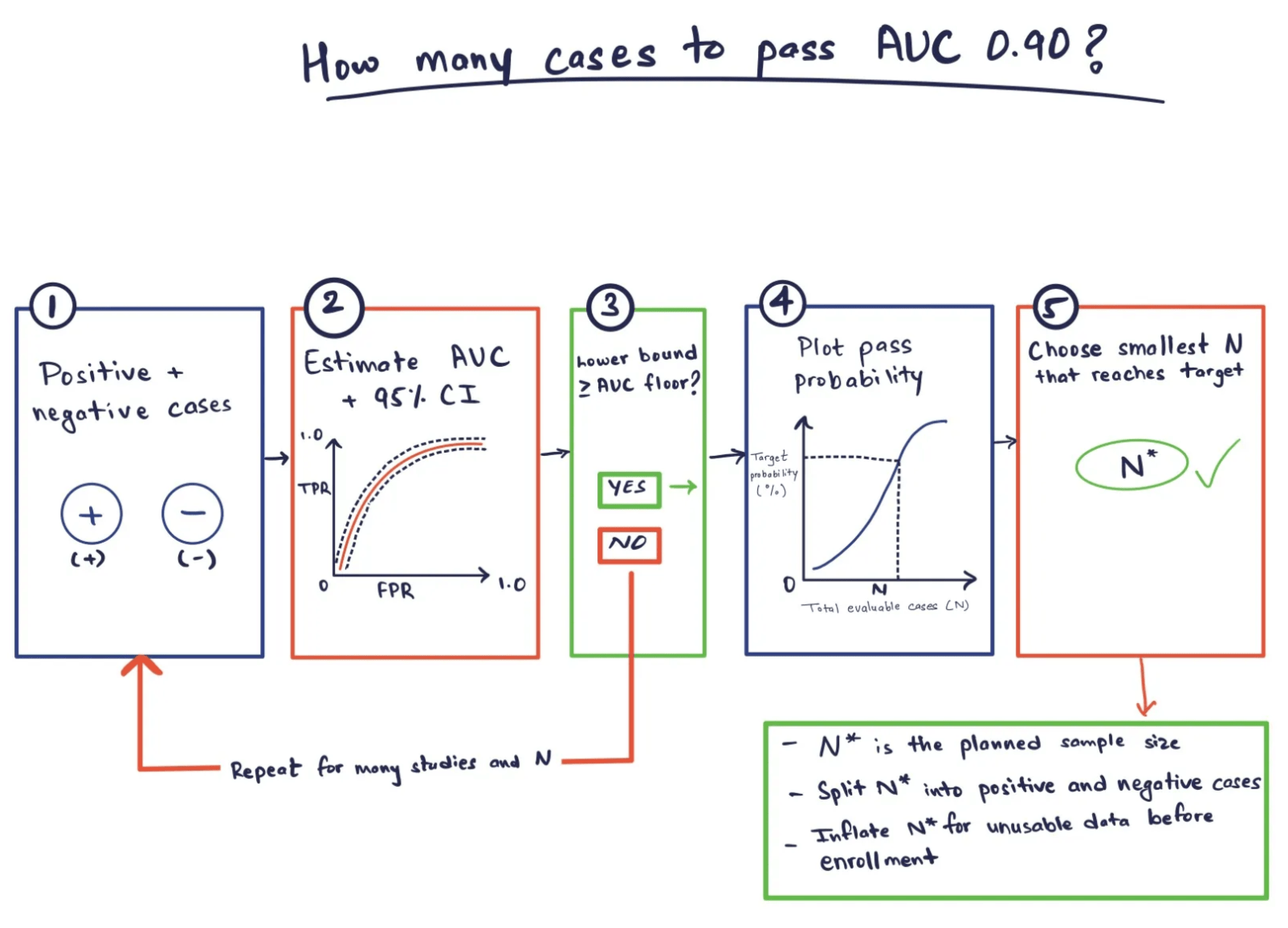
The calculator is intentionally fast. For a pivotal plan, we use it to find a useful search range and then simulate the complete study using the same AUC estimator, confidence interval, missing data rules, and independent unit planned for the final analysis.
Step 1. Translate the acceptance criterion into a pass rule 🔗
For the worked example, a study passes only when the following condition holds.
\[LCL_{95\%}(AUC) \ge 0.90.\]We assume a true AUC of 0.93 and target 80% pass probability.
expected_auc = 0.93
auc_floor = 0.90
target_pass_probability = 0.80
confidence_level = 0.95
positive_fraction = 0.50

print("Planning assumptions")
print(f"  Expected true AUC: {expected_auc:.3f}")
print(f"  Minimum acceptable lower bound: {auc_floor:.3f}")
print(f"  Target probability that the future study passes: {target_pass_probability:.1%}")
print(f"  Confidence interval: two-sided {confidence_level:.0%}")
print(
    f"  Evaluable case mix: {positive_fraction:.0%} positive / "
    f"{1 - positive_fraction:.0%} negative"
)
Output
Planning assumptions
  Expected true AUC: 0.930
  Minimum acceptable lower bound: 0.900
  Target probability that the future study passes: 80.0%
  Confidence interval: two-sided 95%
  Evaluable case mix: 50% positive / 50% negative
Choose an expected AUC that you can justify for the final locked model in the patients and settings where it will be used. Do not plan the study around the highest AUC observed in a small pilot.
Step 2. Get a fast positive/negative case estimate 🔗
The Hanley and McNeil approximation estimates the standard error of one empirical AUC.
\[SE(\widehat{AUC})= \sqrt{\frac{ A(1-A)+(n_+-1)(Q_1-A^2)+(n_--1)(Q_2-A^2) }{n_+n_-}},\]where
\[Q_1=\frac{A}{2-A}, \qquad Q_2=\frac{2A^2}{1+A}.\]Approximating \(\widehat{AUC}\) as normal, the probability of passing is given by
\[P(\text{pass}) \approx \Phi\!\left(\frac{A-A_0}{SE(\widehat{AUC})}-z_c\right),\]where \(A_0=0.90\) and \(z_c=1.96\) for the lower end of a two-sided 95% confidence interval.
import math
from scipy.stats import norm

def auc_se(auc, n_positive, n_negative):
    q1 = auc / (2 - auc)
    q2 = 2 * auc**2 / (1 + auc)
    variance = (
        auc * (1 - auc)
        + (n_positive - 1) * (q1 - auc**2)
        + (n_negative - 1) * (q2 - auc**2)
    ) / (n_positive * n_negative)
    return math.sqrt(variance)

def pass_probability(auc, floor, n_positive, n_negative):
    se = auc_se(auc, n_positive, n_negative)
    return norm.cdf((auc - floor) / se - norm.ppf(0.975))

probability = pass_probability(
    expected_auc,
    auc_floor,
    n_positive=312,
    n_negative=312,
)
status = (
    "MEETS the planning target"
    if probability >= target_pass_probability
    else "DOES NOT MEET the planning target"
)

print("Hanley and McNeil screening result")
print("  Evaluable cases: 624 total (312 positive + 312 negative)")
print(f"  Approximate probability that the future study passes: {probability:.2%}")
print(f"  Planning target: {target_pass_probability:.2%}")
print(f"  Sample-size check: {status}")
Output
Hanley and McNeil screening result
  Evaluable cases: 624 total (312 positive + 312 negative)
  Approximate probability that the future study passes: 80.06%
  Planning target: 80.00%
  Sample-size check: MEETS the planning target
This is why the screening answer is 312 positive plus 312 negative cases.
Step 3. Build a normalized score model 🔗
For a reusable simulation, start with an equal-variance binormal model.
\[S^-\sim\mathcal{N}(0,1), \qquad S^+\sim\mathcal{N}(\delta,1).\]The separation that produces a target AUC is given by
\[\delta=\sqrt{2}\,\Phi^{-1}(AUC).\]For AUC 0.93, \(\delta\approx2.087\). The absolute score scale does not matter for ranking. The overlap does.
import numpy as np
from scipy.stats import norm

rng = np.random.default_rng(20260722)
delta = math.sqrt(2) * norm.ppf(0.93)

positive_scores = rng.normal(delta, 1, 312)
negative_scores = rng.normal(0, 1, 312)
Output
Simulated study generated
  Target population AUC: 0.930
  Binormal score separation: 2.087
  Cases drawn: 624 total (312 positive + 312 negative)
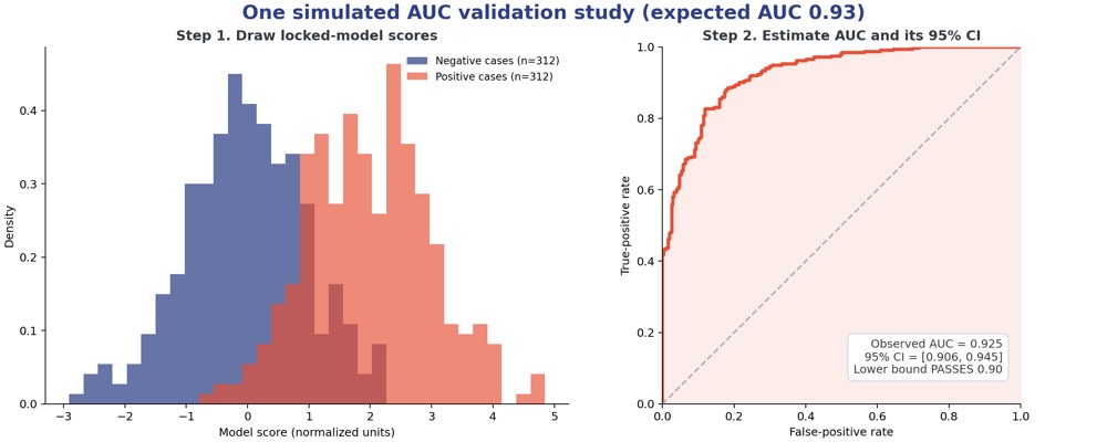
The binormal model is a transparent baseline, not a claim that real scores are normal. Prefer independent pilot distributions, and model unequal variances, ordinal ratings, or clinically important ROC shapes when they matter.
Step 4. Calculate the empirical AUC and its DeLong interval 🔗
DeLong and colleagues estimate AUC variance from the variability of each positive and negative case’s pairwise placements.
def empirical_auc_and_delong_se(positive, negative):
    differences = positive[:, None] - negative[None, :]
    wins = (differences > 0).astype(float) + 0.5 * (differences == 0)
    v10 = wins.mean(axis=1)
    v01 = wins.mean(axis=0)
    auc = wins.mean()
    variance = v10.var(ddof=1) / len(positive) + v01.var(ddof=1) / len(negative)
    return auc, math.sqrt(variance)

auc, se = empirical_auc_and_delong_se(positive_scores, negative_scores)
lower = auc - norm.ppf(0.975) * se
upper = auc + norm.ppf(0.975) * se
passed = lower >= 0.90

print("Result for this one simulated 624-case study")
print(f"  Observed AUC: {auc:.3f}")
print(f"  Raw DeLong 95% confidence interval: [{lower:.3f}, {upper:.3f}]")
print(f"  Acceptance rule: lower confidence bound >= {auc_floor:.3f}")
print(f"  Study result: {'PASS' if passed else 'FAIL'}")
Output
Result for this one simulated 624-case study
  Observed AUC: 0.925
  Raw DeLong 95% confidence interval: [0.906, 0.945]
  Acceptance rule: lower confidence bound >= 0.900
  Study result: PASS
Raw Wald, logit-DeLong, and stratified bootstrap intervals can behave differently near 0 and 1. Simulate the exact interval named in the protocol. “A 95% DeLong interval” is not specific enough.
Step 5. Repeat the entire study across candidate N 🔗
For each candidate count, draw a fresh study, apply the complete pre-specified pass rule, and choose the simulation count from a pre-specified Monte Carlo error target. Ten thousand runs give a 95% Monte Carlo margin of about 0.8 percentage points when the pass probability is 80%, so use more runs when that precision cannot distinguish adjacent candidate sizes. Choose the smallest count whose pass fraction reaches the target.
rng = np.random.default_rng(20260723)

def simulated_pass_probability(n_each, simulations=10_000):
    delta = math.sqrt(2) * norm.ppf(0.93)
    passes = 0
    for _ in range(simulations):
        positive = rng.normal(delta, 1, n_each)
        negative = rng.normal(0, 1, n_each)
        auc, se = empirical_auc_and_delong_se(positive, negative)
        passes += auc - norm.ppf(0.975) * se >= 0.90
    return passes / simulations

for n_each in [125, 250, 312, 417]:
    total = 2 * n_each
    probability = simulated_pass_probability(n_each)
    status = (
        "MEETS the 80% planning target"
        if probability >= target_pass_probability
        else "BELOW the 80% planning target"
    )
    print(
        f"Candidate sample size: {total} total "
        f"({n_each} positive + {n_each} negative)"
    )
    print(f"  Simulated probability that the future study passes: {probability:.2%}")
    print(f"  Planning check: {status}")
    print()
Output
Candidate sample size: 250 total (125 positive + 125 negative)
  Simulated probability that the future study passes: 51.51%
  Planning check: BELOW the 80% planning target

Candidate sample size: 500 total (250 positive + 250 negative)
  Simulated probability that the future study passes: 76.05%
  Planning check: BELOW the 80% planning target

Candidate sample size: 624 total (312 positive + 312 negative)
  Simulated probability that the future study passes: 82.76%
  Planning check: MEETS the 80% planning target

Candidate sample size: 834 total (417 positive + 417 negative)
  Simulated probability that the future study passes: 91.99%
  Planning check: MEETS the 80% planning target
This raw-DeLong simulation crosses 80% before the screening curve. Refine the \(N\) grid near that crossing. At 90% power, 10,000 runs have Monte Carlo 95% uncertainty of about ±0.6 percentage points.
Run the code blocks above in order. The reported outputs were generated with Python 3.9.6, NumPy 2.0.2, SciPy 1.13.1, and Matplotlib 3.9.4. The fixed seed reproduces the four displayed simulation results with those versions. Other NumPy versions can produce different random draws, so compare results within Monte Carlo uncertainty instead of expecting the final decimal to match.
Results and takeaways 🔗
The margin above 0.90 drives the answer 🔗
| Defensible expected AUC | 80% pass probability | 90% pass probability |
|---|---|---|
| 0.91 | 7,190 total (3,595 positive, 3,595 negative) | 9,624 total (4,812 positive, 4,812 negative) |
| 0.92 | 1,600 total (800 positive, 800 negative) | 2,142 total (1,071 positive, 1,071 negative) |
| 0.93 | 624 total (312 positive, 312 negative) | 834 total (417 positive, 417 negative) |
| 0.94 | 302 total (151 positive, 151 negative) | 404 total (202 positive, 202 negative) |
| 0.95 | 162 total (81 positive, 81 negative) | 216 total (108 positive, 108 negative) |
| 0.96 | 92 total (46 positive, 46 negative) | 122 total (61 positive, 61 negative) |
| 0.97 | 52 total (26 positive, 26 negative) | 68 total (34 positive, 34 negative) |
These are screening estimates for the stated normal approximation. They are useful for feasibility and sensitivity analysis, not for selecting a favorable expected AUC after looking at the validation set.
Class imbalance can erase the apparent budget 🔗
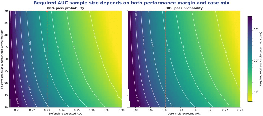
At expected AUC 0.93 and 80% pass probability, the screening estimate follows.
| Positive share of evaluable set | Positive cases | Negative cases | Total evaluable cases |
|---|---|---|---|
| 10% | 278 | 2,502 | 2,780 |
| 20% | 284 | 1,136 | 1,420 |
| 30% | 290 | 677 | 967 |
| 50% | 312 | 312 | 624 |
AUC is invariant to prevalence while the distributions of scores under each class remain unchanged, but it depends on the sizes of both classes. In the case of serial enrollment, prevalence determines the recruitment of the rare stratum. In an enriched study, state fixed quotas and justify the intended-use spectrum.
Work backward from N = 250 budget 🔗
Given 125 positive and 125 negative evaluable cases, an expected AUC of 0.93 and using the same rule of two-sided 95% lower bound, the estimated pass probability is just 42.5%.
For a balanced 250 case budget to provide 80% pass probability, the defensible expected AUC must be about 0.943. For 90%, it must be about 0.948. If only 20% of the 250 cases are positive, expected AUC 0.93 gives only about a 21.6% chance of passing. The expected AUC would need to be about 0.957 for 80% pass probability.
FDA sources cited above do not define the minimum of 250 cases for AUC studies universally. Rather, begin with the stated claim, pass rule, expected performance, and analysis approach, and check whether 250 justifies them.
The confidence interval method changes N 🔗
For the default 0.93 versus 0.90 balanced example, several defensible planning methods give different answers.
| Planning and analysis method | About 80% pass probability | About 90% pass probability |
|---|---|---|
| Hanley and McNeil screening approximation | 624 total | 834 total |
| Equal-binormal simulation, raw DeLong Wald CI | 570 total | 780 total |
| Equal-binormal simulation, logit-DeLong CI | 660 to 670 total | 870 to 880 total |
| Published Shu and Zou confidence-interval assurance formula | 714 total | 954 total |
The Shu and Zou method targets assurance that an AUC interval excludes an unacceptable value. The spread is a reason to pre-specify and simulate rather than select the smallest result. Obuchowski showed that the Hanley and McNeil approach can underestimate sample size for some rating distributions and variance ratios.
What a reviewer ready plan should address 🔗
A reviewer ready plan should answer eight questions.
- What must clear 0.90? Identify the point estimate or confidence bound criterion, whether the confidence bound is one-sided or two-sided, and what the interval is. The one-sided 95% confidence bound is defined by 1.645, not 1.96. Using the default screening example, this reduces the 80% estimated needed sample size from 624 to 492 cases.
- Why is the expected AUC credible? Trace it to locked model pilot data, an appropriate predicate, or comparable literature, and show sensitivity analyses.
- How many cases are independently evaluable? Provide separately positive and negative quotas of evaluable cases. Then account for the number reduction caused by non-evaluable cases. Positive vs negative comparison is not independent patient units.
- Does the case spectrum match intended use? Include relevant severities, mimics, sites, equipment, protocols, demographics, and user conditions. In CADe reader studies, FDA warns that enrichment may affect reader performance and can introduce bias.
- Was the model and workflow locked? Pre-specify the score direction, tie handling, analysis population, missing-result rules, and transformations before unblinding.
- Is the patient the independent unit? Account for the correlation among multiple images, lesions, organs, specimens, or frames of the same patient via patient resampling or design specific model.
- Is this a reader study? Standalone DeLong calculations do not size a multi-reader, multi-case claim. Model reader and case effects. FDA’s iMRMC software supports correlated MRMC sizing and analysis.
- Does global AUC support the clinical claim? Also report clinically relevant operating-point metrics. A strong global AUC does not guarantee adequate sensitivity or specificity where the device will operate.
Frequently asked questions 🔗
How many cases are needed to show that the AUC lower confidence bound clears 0.90?
Under one common screening design with expected AUC 0.93, equal positive and negative counts, independent patients, the lower end of a two-sided 95% interval at least 0.90, and 80% pass probability, the Hanley and McNeil approximation gives about 624 evaluable cases. The final number changes with the expected AUC, confidence-interval method, class mix, clustering, and target pass probability.
Can a true AUC of 0.90 reliably pass a 0.90 lower confidence bound?
No, not with a correctly calibrated lower confidence bound at those assurance levels. If the true AUC equals the floor, increasing sample size makes the interval narrower around 0.90 but does not move the truth above 0.90. Under large sample calibration, the chance that the lower end of a two-sided 95% interval exceeds the true value approaches 2.5%, not 80% or 90%.
Does disease prevalence affect ROC AUC sample size?
Prevalence does not change the population AUC when the positive and negative score distributions stay the same. It does change how many positive and negative cases appear in a consecutive test set, and therefore changes AUC precision and total enrollment. Plan the two evaluable strata explicitly.
Are 250 cases enough for an AUC study?
Not automatically. With 125 positive and 125 negative cases, expected AUC 0.93, and the lower end of a two-sided 95% interval required to clear 0.90, the screening approximation gives only about a 42.5% chance of passing. The same 250 case budget reaches about 80% only when expected AUC is roughly 0.943 under those assumptions.
Conclusion 🔗
Required number of cases is highly determined by margin above the floor and complete pass rule. Absolute AUC contributes to the variance. For a balanced expected AUC 0.93, an approximate answer for 80% pass probability is around 624 evaluable cases, not a universal final answer.
Make your estimator and confidence interval fixed, validate expected score distributions, make sure that you have true independent unit, simulate complete analysis, split the result into positive and negative quotas. When the budget does not allow you to do all of that in the 250 case set, adjust your claim, optimize expected performance, enrich responsibly, or discuss another design before collecting a pivotal set in order to avoid missing 0.90 on the lower bound.
If you want a second set of eyes before a Pre-Sub or pivotal collection, contact Innolitics. We review the acceptance criterion, score model, test-set composition, reference standard, and statistical analysis together because they determine the sample size together.
Sources 🔗
- Hanley JA, McNeil BJ. AUC meaning and use. Radiology. 1982.
- DeLong ER, DeLong DM, Clarke-Pearson DL. Nonparametric comparison of correlated ROC AUCs. Biometrics. 1988.
- Obuchowski NA. ROC study sample-size computation. Investigative Radiology. 1994.
- Shu D, Zou G. ROC sample-size planning with precision and assurance. Statistical Methods in Medical Research. 2023. Open preprint.
- FDA. Final diagnostic-test statistical guidance. 2007.
- FDA. Final radiology CADe clinical-performance guidance. 2022.
- FDA. Draft AI-enabled device software guidance. 2025.
- FDA. iMRMC software for multi-reader multi-case studies. 2025.