
Sensitivity and specificity sample size: the short answer 🔗
If your protocol says, “We will validate the device on 250 patients,” expect the first statistical question to be 250 what?
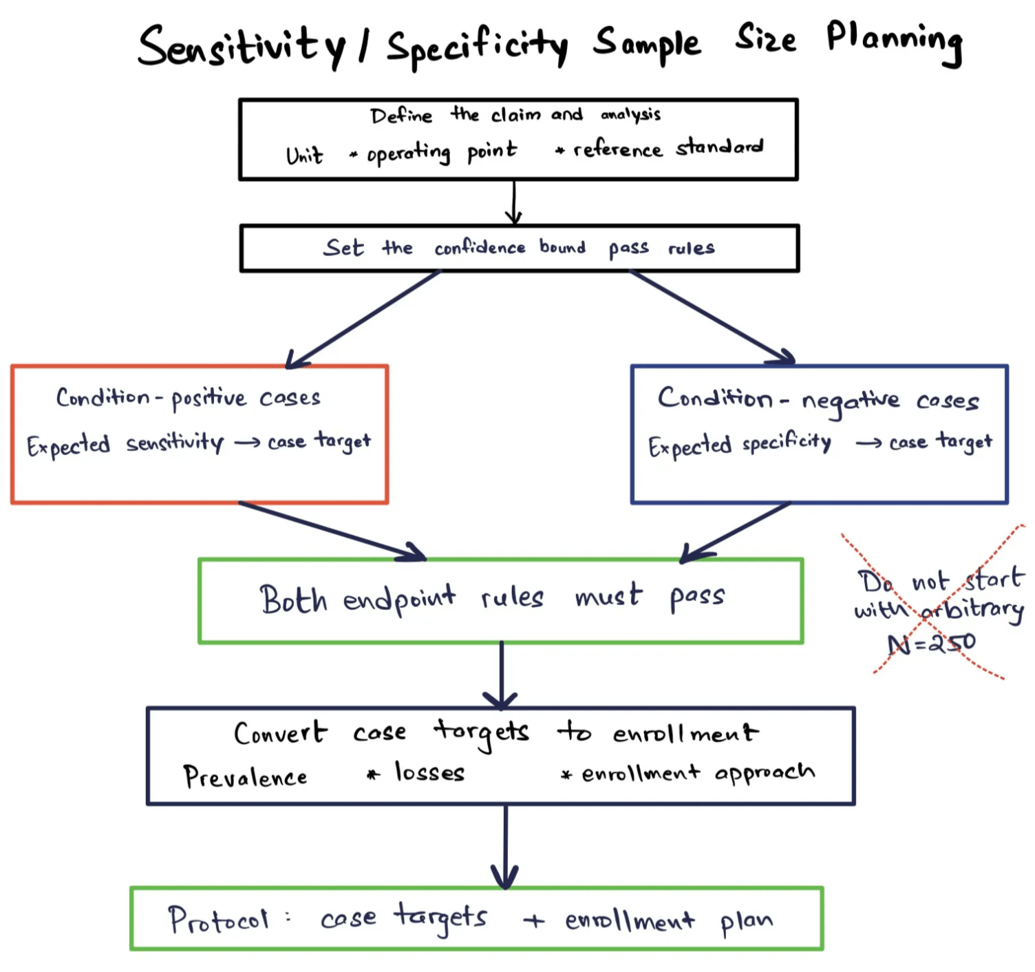
- Sensitivity is powered by the number of patients who have the target condition: \(n_+ = TP + FN\).
- Specificity is powered by the number of patients who do not have the target condition: \(n_- = TN + FP\).
- Total enrollment depends on how many of each you need, the condition prevalence in the study population, any enrichment, and the pre-specified non-evaluable loss rate.
The FDA does not have a universally applicable regulation stating that a particular sensitivity and specificity study should enroll 100, 250, or 500 patients. The specific guidance for a certain device, special controls, risk associated with the claim, and previous FDA feedback on the matter can provide the number to shoot at. Otherwise, it's up to you to link the claim to an adequately specified pass criterion and then demonstrate that the specified number of positives/negatives is likely to result in the study being passed when the device works as intended.
FDA's final 2025 guidance for AI-enabled device PCCPs is unusually clear on the matter. Its performance-evaluation checklist includes questions about how sample size was determined, the tradeoff between sensitivity and specificity, management of the reference standard and missing data, and the clinical rationale for the acceptance criteria. This checklist was written for modifications to AI-enabled devices through a PCCP. It does not represent a universal checklist for every initial submission. Nevertheless, it closely resembles the set of questions one might encounter during a performance plan stress test.
Small, seemingly perfect studies demonstrate the importance of the denominator size. An FDA-authored paper provides the following example: 5/5 correct gives 100% sensitivity, but the lower end of its two-sided 95% score interval is only 56.6%. Even 30/30 only raises the lower end of the two-sided 95% score interval to 88.6%.
Our recommendation is simple, “Write the reviewer answer before collecting the first case”.
Start with the pass rule, not a sample size formula 🔗
Sensitivity and specificity are binomial proportions:
\[\widehat{Se}=\frac{TP}{TP+FN}, \qquad \widehat{Sp}=\frac{TN}{TN+FP}.\]A point estimate alone generally does not make for a good acceptance criterion. Having 90% sensitivity in 20 cases that have the condition present is different from having 90% sensitivity in 200 cases. FDA guidelines on diagnostic testing mention that sensitivity and specificity should be presented along with confidence intervals.
For a binary standalone performance study, a clean demonstration rule is:
\[LCL_{95\%}(Se) \ge Se_{min} \quad \textbf{and} \quad LCL_{95\%}(Sp) \ge Sp_{min}.\]This is just one example of a good design choice that is not a mandatory FDA requirement. Instead, your medical device could require a precision target, comparison, non-inferiority to a predicate, MRMC analysis, or a custom design for the device. In case of a method comparison claim based on a continuous output procedure, a different design problem arises, which is covered by our Bland–Altman sample size guidelines.
If you plan to apply a one-sided lower confidence limit, state this clearly. A one-sided 95% lower confidence limit is numerically different from the lower limit of a two-sided 95% confidence interval. Below are a calculator and an example of the latter.
Precision and conditional power answer different questions 🔗
A common quick calculation chooses the number of condition-positive and condition-negative cases to target a confidence-interval half-width \(d\):
\[n_+ \approx \frac{z_{1-\alpha/2}^2 Se(1-Se)}{d_{Se}^2}, \qquad n_- \approx \frac{z_{1-\alpha/2}^2 Sp(1-Sp)}{d_{Sp}^2}.\]This is a precision design. The question asked here is, "How precise should the estimate be?"
The calculator below uses a conditional power design. It asks, “If true performance equals our defensible expectation, what case count gives us at least a 90% chance that both lower confidence bounds clear their acceptance floors?” That is usually closer to the business and regulatory question when your protocol has a pass/fail criterion.
Exact sensitivity and specificity sample size calculator 🔗
The defaults are an illustrative AI/ML SaMD scenario : expected sensitivity of 0.90, expected specificity of 0.92, lower-bound acceptance floors of 0.80, and a 90% target chance that both endpoints pass. They are useful starting values from our analysis of AI/ML SaMD acceptance criteria, not recommendations for every device.
Interactive planning tool
Sensitivity / specificity sample-size planner
Exact two-sided 95% Clopper–Pearson lower bounds. The result is a planning aid, not an FDA determination.
Condition-positive target
—
Condition-negative target
—
Mean-yield enriched estimate
—
Expected total when positive and negative strata are collected separately, including the entered loss rate. Continue until both evaluable quotas are met.
Consecutive enrollment estimate
—
Expected total at the entered prevalence and loss rate. Random prevalence means this is not a guarantee.
The calculator treats the positive and negative strata as fixed and independent. To target a 90% chance that both endpoints pass, it targets \(\sqrt{0.90}=94.87\%\) conditional power for each endpoint. If independence is not defensible, use a more conservative joint-error allocation or simulate the complete design.
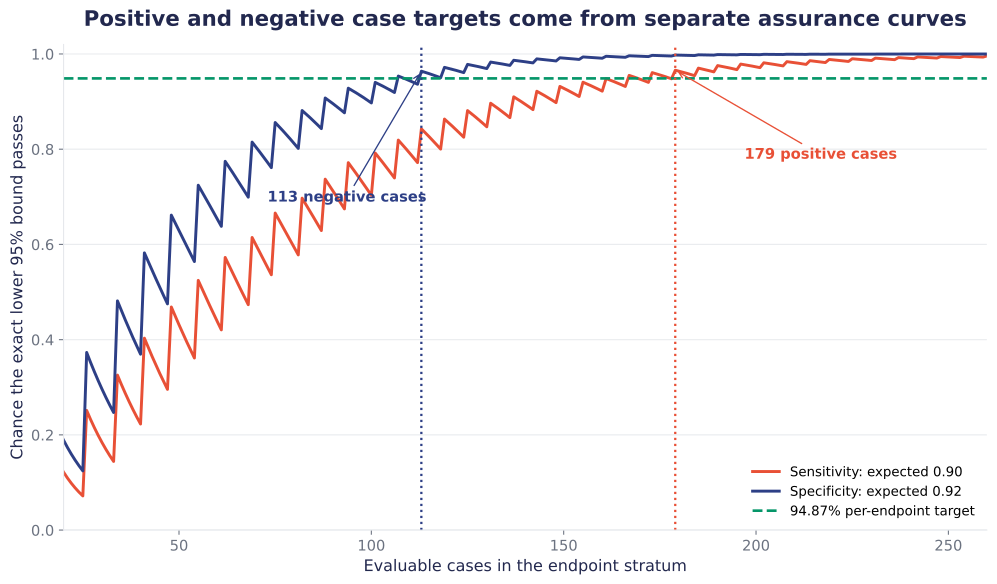
Because exact-binomial power is saw-toothed, this walkthrough uses a conservative monotone-safe quota, the first count for which every larger count through n_max=10,000 also meets the endpoint target. The pointwise first-passing counts are 167 positive and 107 negative cases, but some immediately larger counts fall below target. This convention is a planning choice, not an FDA requirement.
Worked example : Why a 250 patient budget may fail 🔗
With the calculator defaults, the targets will be:
- 179 condition-positive patients for sensitivity. This requires a minimum of 154 true positives to ensure the exact lower 95% bound exceeds 0.80.
- 113 condition-negative patients for specificity. This requires a minimum of 99 true negatives to ensure the exact lower 95% bound exceeds 0.80.
- 292 evaluable patients in the directly filled positive and negative strata.
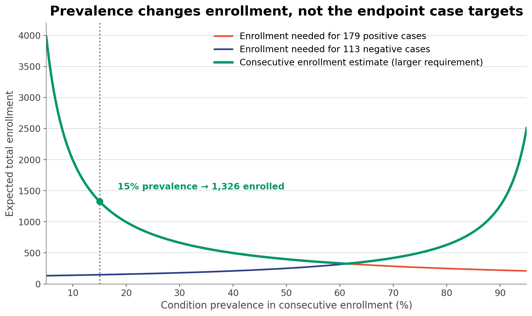
Allowing for 10% loss, the mean-yield enriched estimate is 325 patients. In a consecutive design with 15% condition prevalence, sensitivity is limiting and the mean-yield enrollment estimate is 1,326 patients. If enrollment must be fixed, 1,445 patients gives about a 90% probability of obtaining at least 179 evaluable positive cases under the same simple yield assumptions.
Consider now a budget of 250 patients. With 10% losses, this budget leads to roughly 225 evaluable patients. At 15% prevalence, the expected numbers are 33.75 condition-positive and 191.25 condition-negative patients. Specificity may be well covered, but sensitivity is short by 145.25 positive patients, or about 145.
These are the four numbers that belong in the protocol:
| Number reviewers need | What it answers | Worked example |
|---|---|---|
| Evaluable condition-positive cases | Is sensitivity adequately supported? | 179 |
| Evaluable condition-negative cases | Is specificity adequately supported? | 113 |
| Mean-yield enriched estimate | How many cases are collected when both strata are filled directly, including losses? | 325 |
| Consecutive enrollment estimate | How many patients are expected at the planned prevalence and loss rate? | 1,326 |
Do not label all four numbers “sample size.” Each answers a different question.
This does not inherently make the study impossible to do. Rather, it means that a choice must be made prior to setting the protocol in stone:
- Enrich with condition-positive cases. This is efficient, but preserve the intended-use range and note how enrichment affects prevalence-dependent statistics and case difficulty.
- Improve expected performance of the device. Expected sensitivity well above its minimum is much more effective at decreasing the number of positive cases needed.
- Change the claim or acceptance criteria only when supported by evidence. Predicate performance and other relevant evidence may inform the justification, together with special controls, risk assessment, and Pre-Sub feedback. Cost alone cannot.
- Expand enrollment or reconfigure the study design. Multisite retrospective data collection might be the least cumbersome feasible path forward for a rare condition.
Wrong choices include maintaining “N=250” in the protocol and hoping the final confidence interval ends up working.
What FDA Reviewers Will Ask 🔗
1. What exactly must pass? 🔗
Identify estimand, analysis population, operating point, interval procedure, confidence level, and inequality. "Sensitivity will exceed 0.80" is not a proper statement. "The lower limits of the specified two-sided 95% exact binomial CIs for patient-level sensitivity and specificity will each be no less than 0.80" is checkable.
When both sensitivity and specificity must pass, consider the success criteria jointly. Under independence, two success criteria with 90% power each have about 81% joint power.
2. Why are the expected rates and minimums credible? 🔗
Both your expected sensitivity and specificity will determine the sample size just as the acceptance floors do. Make sure they are determined using pilot studies with fixed algorithms, a suitable predicate, literature on a similar target population, special controls, or other valid evidence. Do not use final test results to determine the values.
Acceptance criteria should be clinically justified in light of the intended use, the consequences of false-negative and false-positive results, and other relevant evidence. Because those consequences are often unequal, symmetric acceptance floors are not automatically appropriate.
3. How many positive and negative cases will be evaluable? 🔗
Show \(n_+\) and \(n_-\) separately. Then show how total enrollment produces both:
\[N_{enroll} \approx \frac{1}{1-r} \max\left(\frac{n_+}{\pi},\frac{n_-}{1-\pi}\right),\]where \(\pi\) is the expected condition-positive fraction in the enrolled study flow and \(r\) is the pre-specified non-evaluable loss rate. This is an expectation, not a guarantee. The protocol could alternatively specify a minimum number of evaluable subjects for each stratum and collect data until both numbers are reached.
4. Does the study population match the intended use? 🔗
FDA guidance for diagnostic tests warns about spectrum bias, including only easy positive cases and clear negative controls can make both measures overly optimistic. Consider relevant disease severities, imitators, confounders, demographics, sites, instrumentation, acquisition methods, and use conditions.
Enrichment is not inherently bad. FDA’s 2022 CADe guidance mentions enrichment explicitly as one possibility for an efficient study design. At the same time, it warns about changing reader performance and potential bias from enrichment. Describe the selection criteria, and do not select cases based on how well your system performs on them.
5. Is “sensitivity/specificity” the correct terminology? 🔗
To report diagnostic sensitivity and specificity directly, condition status generally must be established using a designated reference standard; it need not be a perfect “gold standard.” When the new test is compared only with a non-reference comparator, including a predicate that is not itself a reference standard FDA recommends positive percent agreement (PPA) and negative percent agreement (NPA) rather than sensitivity and specificity. Increasing sample size alone will not correct bias caused by reference-standard error or by incorporating the candidate test into the reference-standard determination.
Explain who determined the “truth,” what information the determination was based on, and how disagreements or uncertain reference-standard results were resolved. Was the device output part of that reconciliation?
6. What is the independent unit? 🔗
Ten lesions in one patient are not automatically ten independent sensitivity observations. Neither are repeated images, video frames, multiple readers, bilateral organs, or several specimens from the same subject. If the claim is patient-level, the patient count is usually the primary denominator.
For clustered data, use an analysis and power method that preserves the correlation structure, such as cluster bootstrap, GEE, mixed models, or a design-specific simulation. For reader-aided claims, a standalone binomial calculation does not replace an MRMC study design.
7. Was the operating point locked before testing? 🔗
Sensitivity and specificity trade off against each other. If you pick the threshold after inspecting the test set, it uses information from the test set and makes the confidence interval too optimistic. Set the threshold and all other factors, such as device version, intended use, pre-processing, scoring algorithm, and acceptance criteria, prior to the pivotal trial.
If you plan to claim multiple thresholds, results, device versions, endpoints, or populations, pre-specify the testing strategy, address multiplicity as applicable, and identify the smallest relevant denominator.
8. What happens to invalid, indeterminate, and missing results? 🔗
FDA’s diagnostic-test guidance states that discarding equivocal results will likely bias performance estimates. Pre-specify how device failures, low-quality inputs, ambiguous outputs, protocol deviations, missing reference values, and repeat tests will be handled in the primary analysis. Differentiate between an intention-to-diagnose analysis and a per-protocol analysis, and account for every enrolled patient.
Increasing the sample size to cover 10% loss is only helpful when 10% seems realistic. It doesn’t mean that you are allowed to drop problematic patients silently.
9. Can important subgroups still be interpreted? 🔗
Overall study power does not guarantee meaningful confidence intervals within subgroups of sex, age, race, disease severity, site, scanner, or acquisition protocol. Important cohorts should support appropriate characterization, but subgroup powering is generally unnecessary unless a subgroup claim or known difference makes it necessary. FDA's 2025 sex-specific guidance recommends sex-specific analyses of diagnostic performance while noting that subgroup analysis may not be warranted when overall diagnostic accuracy is very high.
Specify upfront which subgroup analyses are confirmatory, which are descriptive, and when pooling is appropriate.
A reviewer ready sensitivity and specificity sample size justification 🔗
For the worked example, the core protocol language could fit in three short paragraphs:
Primary endpoints and success criterion. The primary analysis will provide estimates of patient-level sensitivity and specificity at the locked operating point. Success will mean that the lower bounds of the pre-specified two-sided 95% exact binomial confidence intervals for sensitivity and specificity are each at least 0.80.
Case targets and collection. With the assumed true sensitivity of 0.90, true specificity of 0.92, and 90% joint conditional-power target under fixed and independent positive and negative strata, the study needs at least 179 condition-positive and 113 condition-negative evaluable patients. Accounting for 10% non-evaluable loss, the mean-yield enriched estimate is 325 patients. Given 15% condition prevalence in a consecutive cohort, the mean-yield enrollment estimate is 1,326 patients. If enrollment must be fixed, 1,445 patients gives about a 90% probability of filling the 179 positive quota under the same simple yield assumptions. For quota-based accrual, collection continues until both minimum evaluable stratum sizes are attained. A fixed-enrollment protocol instead follows its pre-specified total and accrual-monitoring rules.
Analysis protections. The reference-standard procedure, analysis unit, operating point, handling of missing and indeterminate results, and clinically important subgroup analyses will be defined before the test-set evaluation.
These numbers serve as an illustration. Do not copy and paste them into a protocol if your device does not match the assumptions used here. What is important is the logical sequence: claim → pass rule → expected performance → positive and negative case targets → total enrollment → analysis protections.
Reproducible Python Implementation 🔗
This implementation uses the same rule as the web calculator. It returns the first monotone-safe case count whose endpoint power remains at or above target for every larger count through n_max.
Run the code blocks in order in one Python session or notebook. The displayed outputs were independently reproduced with Python 3.9.6, NumPy 2.0.2, SciPy 1.13.1, and Matplotlib 3.9.4.
Step 1: Check a small perfect-looking study 🔗
from dataclasses import dataclass
from math import ceil, sqrt

import matplotlib.pyplot as plt
import numpy as np
from scipy.stats import beta, binom

CONFIDENCE = 0.95
ALPHA_TAIL = (1 - CONFIDENCE) / 2

def exact_lower_bound(successes, cases):
    """Lower end of a two-sided Clopper-Pearson interval."""
    if successes == 0:
        return 0.0
    return beta.ppf(ALPHA_TAIL, successes, cases - successes + 1)

def required_successes(cases, minimum):
    """Smallest success count whose exact lower bound clears minimum."""
    return int(binom.isf(ALPHA_TAIL, cases, minimum)) + 1

successes = required_successes(cases=30, minimum=0.80)
power = binom.sf(successes - 1, 30, 0.90)

print(f"30/30 exact lower bound: {exact_lower_bound(30, 30):.3f}")
print(f"Required to clear 0.80: {successes}/30")
print(f"Power when true sensitivity is 0.90: {power:.1%}")
Output:
30/30 exact lower bound: 0.884
Required to clear 0.80: 29/30
Power when true sensitivity is 0.90: 18.4%
This shows why 30 positive cases are not automatically enough.
Step 2: Calculate the sensitivity target 🔗
@dataclass(frozen=True)
class EndpointPlan:
    cases: int
    required_successes: int
    power_at_cases: float
    lower_ci_at_successes: float

def exact_endpoint_plan(
    expected,
    minimum,
    endpoint_power,
    confidence=0.95,
    n_max=10_000,
):
    """Return the first count whose power stays at target through n_max."""
    if not 0 < minimum < expected < 1:
        raise ValueError("Require 0 < minimum < expected < 1")
    if not 0 < endpoint_power < 1:
        raise ValueError("Require 0 < endpoint_power < 1")
    if not 0 < confidence < 1:
        raise ValueError("Require 0 < confidence < 1")

    alpha_tail = (1 - confidence) / 2
    case_counts = np.arange(1, n_max + 1)
    successes = binom.isf(alpha_tail, case_counts, minimum).astype(int) + 1
    power = binom.sf(successes - 1, case_counts, expected)

    # Exact-binomial power is saw-toothed. Require every later count
    # through n_max to meet the endpoint target.
    tail_min_power = np.minimum.accumulate(power[::-1])[::-1]
    candidates = np.flatnonzero(tail_min_power >= endpoint_power)
    if len(candidates) == 0:
        raise ValueError(f"No monotone-safe solution through n={n_max}")

    i = int(candidates[0])
    n = int(case_counts[i])
    k = int(successes[i])
    return EndpointPlan(
        cases=n,
        required_successes=k,
        power_at_cases=float(power[i]),
        lower_ci_at_successes=float(beta.ppf(alpha_tail, k, n - k + 1)),
    )

joint_target = 0.90  # Illustrative planning choice, not an FDA rule
endpoint_target = sqrt(joint_target)

sensitivity = exact_endpoint_plan(
    expected=0.90,
    minimum=0.80,
    endpoint_power=endpoint_target,
)
print(sensitivity)
Output:
EndpointPlan(cases=179, required_successes=154,
             power_at_cases=0.9659, lower_ci_at_successes=0.8008)
The sensitivity target is 179 evaluable condition-positive cases, with at least 154 true positives.
Step 3: Calculate the specificity target and joint power 🔗
specificity = exact_endpoint_plan(
    expected=0.92,
    minimum=0.80,
    endpoint_power=endpoint_target,
)
joint_power = sensitivity.power_at_cases * specificity.power_at_cases

print(specificity)
print(f"Joint power at returned counts: {joint_power:.1%}")
Output:
EndpointPlan(cases=113, required_successes=99,
             power_at_cases=0.9639, lower_ci_at_successes=0.8009)
Joint power at returned counts: 93.1%
The specificity target is 113 evaluable condition-negative cases, with at least 99 true negatives. Under fixed and independent strata, the probability that both endpoints pass at the returned counts is 93.1%.
def endpoint_power_curve(expected, minimum, n_max=250):
    n = np.arange(1, n_max + 1)
    k = binom.isf(ALPHA_TAIL, n, minimum).astype(int) + 1
    return n, binom.sf(k - 1, n, expected)

n_se, power_se = endpoint_power_curve(0.90, 0.80)
n_sp, power_sp = endpoint_power_curve(0.92, 0.80)

plt.figure(figsize=(10, 6))
plt.plot(n_se, 100 * power_se, color="#E85036",
         label="Sensitivity: expected 0.90")
plt.plot(n_sp, 100 * power_sp, color="#2D3F86",
         label="Specificity: expected 0.92")
plt.scatter(179, 100 * sensitivity.power_at_cases, color="#E85036")
plt.scatter(113, 100 * specificity.power_at_cases, color="#2D3F86")
plt.axhline(100 * endpoint_target, color="#059669", linestyle="--",
            label="94.87% power per endpoint")
plt.xlim(20, 250)
plt.ylim(0, 101)
plt.xlabel("Evaluable cases in the endpoint stratum")
plt.ylabel("Probability the exact lower bound passes (%)")
plt.title("Positive and negative case targets are calculated separately")
plt.grid(axis="y", alpha=0.25)
plt.legend()
plt.tight_layout()
plt.show()
Step 4: Translate the case targets into enrollment 🔗
prevalence = 0.15
loss_positive = 0.10
loss_negative = 0.10

positive_to_collect = ceil(
    sensitivity.cases / (1 - loss_positive)
)
negative_to_collect = ceil(
    specificity.cases / (1 - loss_negative)
)
enriched_mean_total = positive_to_collect + negative_to_collect

expected_consecutive = ceil(max(
    sensitivity.cases / (prevalence * (1 - loss_positive)),
    specificity.cases / ((1 - prevalence) * (1 - loss_negative)),
))

# If enrollment must be fixed, power the accrual of the limiting stratum too.
positive_yield = prevalence * (1 - loss_positive)
fixed_enrollment_90 = next(
    n for n in range(expected_consecutive, 10_000)
    if binom.sf(sensitivity.cases - 1, n, positive_yield) >= 0.90
)

print(f"Mean-yield enriched estimate: {enriched_mean_total}")
print(f"Expected consecutive enrollment: {expected_consecutive}")
print(f"90% probability of filling the positive quota: {fixed_enrollment_90}")
Output:
Mean-yield enriched estimate: 325
Expected consecutive enrollment: 1326
90% probability of filling the positive quota: 1445
The values 325 and 1,326 are mean-yield estimates, not guaranteed fixed sample sizes. Collection should continue until both evaluable quotas are met. If enrollment must be fixed, 1,445 gives about a 90% probability of obtaining at least 179 evaluable positive cases under the same simple yield assumptions.
prevalence_grid = np.linspace(0.05, 0.95, 181)
positive_driven = sensitivity.cases / (
    prevalence_grid * (1 - loss_positive)
)
negative_driven = specificity.cases / (
    (1 - prevalence_grid) * (1 - loss_negative)
)

plt.figure(figsize=(10, 6))
plt.plot(100 * prevalence_grid, positive_driven, color="#E85036",
         label="Enrollment needed for 179 positive cases")
plt.plot(100 * prevalence_grid, negative_driven, color="#2D3F86",
         label="Enrollment needed for 113 negative cases")
plt.plot(
    100 * prevalence_grid,
    np.maximum(positive_driven, negative_driven),
    color="#059669",
    linewidth=3,
    label="Consecutive enrollment estimate",
)
plt.axvline(15, color="#737373", linestyle=":")
plt.scatter(15, expected_consecutive, color="#059669")
plt.annotate("15% prevalence → 1,326 enrolled",
             (15, expected_consecutive), xytext=(25, 15),
             textcoords="offset points", color="#059669")
plt.xlim(5, 95)
plt.ylim(0, 4200)
plt.xlabel("Condition prevalence in consecutive enrollment (%)")
plt.ylabel("Expected total enrollment")
plt.title("Prevalence changes enrollment, not the endpoint case targets")
plt.grid(axis="y", alpha=0.25)
plt.legend()
plt.tight_layout()
plt.show()
Step 5: Check a 250-patient budget 🔗
budget = 250
retention = 0.90
expected_positive = budget * retention * prevalence
expected_negative = budget * retention * (1 - prevalence)

print(f"Expected evaluable positive cases: {expected_positive:.2f}")
print(f"Expected evaluable negative cases: {expected_negative:.2f}")
print(f"Expected positive-case shortfall: "
      f"{sensitivity.cases - expected_positive:.2f}")
Output:
Expected evaluable positive cases: 33.75
Expected evaluable negative cases: 191.25
Expected positive-case shortfall: 145.25
The expected condition-positive count is 145.25 below the 179 case target; because 33.75 is an expected count, it does not imply a guaranteed integer shortfall.
The 250 subject budget calculation produces 33.75 expected evaluable condition-positive subjects and a 145.25 case expected shortfall relative to the 179-case sensitivity quota. The 179/113 quotas and 325/1,326 planning values come from Steps 2–4, not from this budget check.
Precomputed Case Count Table 🔗
The table below applies to either endpoint where each cell is an evaluable condition-positive quota for sensitivity or an evaluable condition-negative quota for specificity, not total enrollment. It uses the lower endpoint of a two-sided 95% Clopper–Pearson interval and 94.87% endpoint design power under assumed true performance, corresponding to a 90% joint target for fixed and independent strata. Values are monotone-safe through n_max=10,000. Here em dash means expected performance does not exceed the floor, so no finite solution exists under this design.
| Expected performance | Minimum 0.70 | Minimum 0.75 | Minimum 0.80 | Minimum 0.85 | Minimum 0.90 |
|---|---|---|---|---|---|
| 0.80 | 256 | 929 | — | — | — |
| 0.85 | 105 | 220 | 776 | — | — |
| 0.90 | 53 | 89 | 179 | 595 | — |
| 0.95 | 31 | 44 | 69 | 127 | 387 |
| 0.98 | 22 | 27 | 34 | 56 | 114 |
The following code produces the chart:
floors = [0.70, 0.75, 0.80, 0.85, 0.90]
colors = ["#059669", "#2D3F86", "#E85036", "#7A5195", "#C58A00"]

plt.figure(figsize=(10, 6))
for floor, color in zip(floors, colors):
    expected_grid = np.arange(floor + 0.01, 0.991, 0.005)
    required_n = []
    for expected in expected_grid:
        try:
            plan = exact_endpoint_plan(expected, floor, endpoint_target)
            required_n.append(plan.cases)
        except ValueError:
            required_n.append(np.nan)

    plt.plot(
        100 * expected_grid,
        required_n,
        color=color,
        label=f"Minimum lower bound {floor:.2f}",
    )

plt.scatter(90, 179, color="#E85036", s=60, zorder=5)
plt.annotate(
    "Worked example 0.90 → 179 cases",
    xy=(90, 179),
    xytext=(87.4, 430),
    textcoords="data",
    ha="center",
    va="center",
    arrowprops={
        "arrowstyle": "->",
        "color": "#E85036",
        "linewidth": 1.4,
        "connectionstyle": "arc3,rad=-0.18",
    },
    bbox={
        "boxstyle": "round,pad=0.35",
        "facecolor": "white",
        "edgecolor": "#E85036",
        "alpha": 0.97,
    },
    color="#E85036",
    fontsize=11,
    zorder=6,
)
plt.yscale("log")
plt.xlim(71, 99)
plt.ylim(10, 10_000)
plt.xlabel("Expected sensitivity or specificity (%)")
plt.ylabel("Required evaluable cases (log scale)")
plt.title("Required sample size rises sharply near the acceptance floor")
plt.grid(axis="y", which="both", alpha=0.25)
plt.legend()
plt.tight_layout()
plt.show()
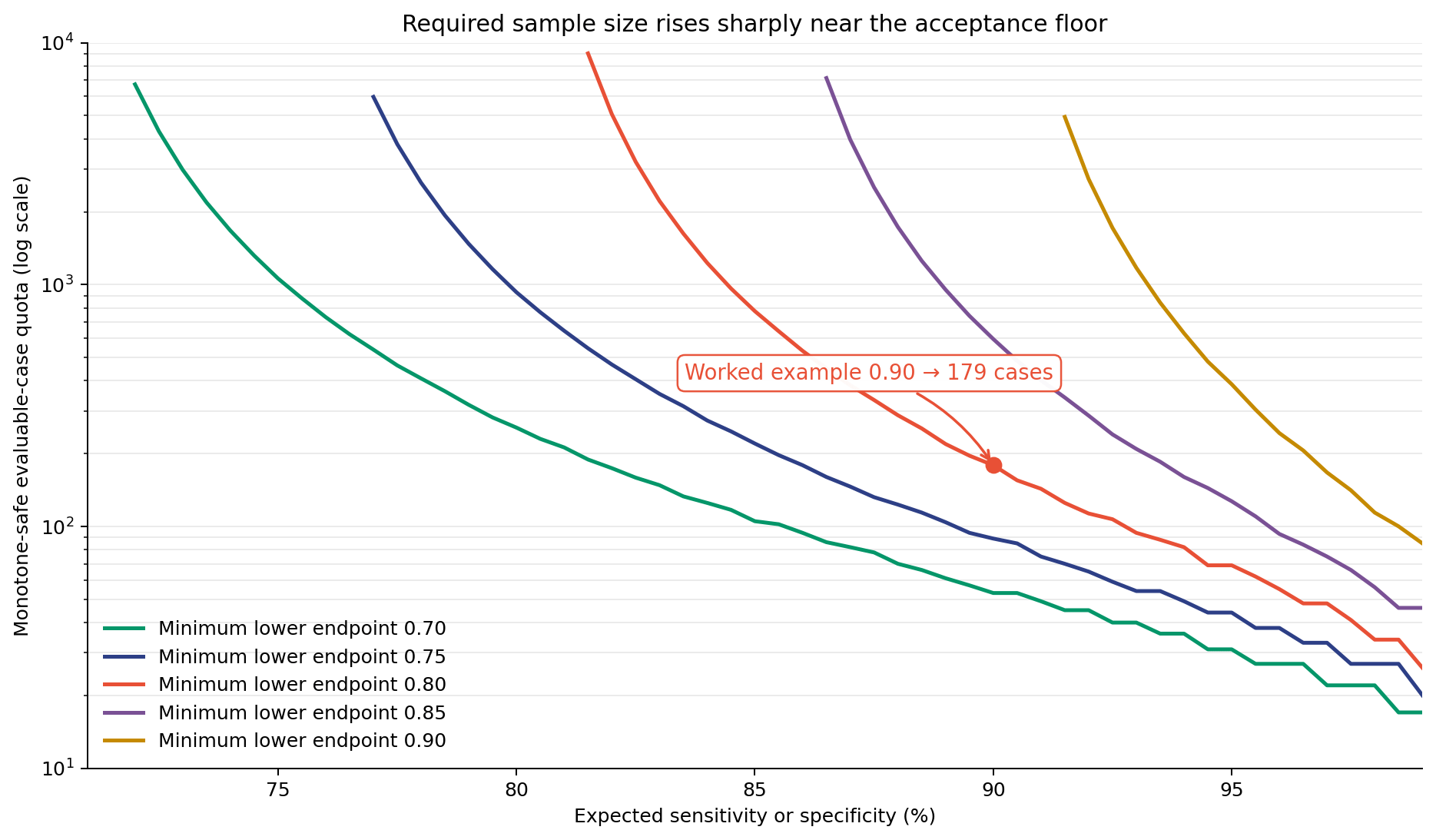
What matters is the “cliff.” When expected performance exceeds the acceptance floor by only five percentage points, several hundred cases may be needed. Better performance reduces the required case count, but it should not be an optimistic assumption inserted merely to fit the budget.
Frequently asked questions 🔗
How many patients do I need to estimate sensitivity and specificity?
There is no single total. Calculate the required condition-positive cases for sensitivity and condition-negative cases for specificity separately. Then translate those targets into enrollment using prevalence, enrichment, and the expected non-evaluable rate. The larger translated requirement drives the consecutive-study total.
Does FDA require at least 250 patients?
No universal FDA rule sets 250 as the minimum for every sensitivity/specificity study. Device-specific guidance, a special control, a predicate, a risk profile, or prior FDA feedback may support a particular count. FDA will care whether the positive and negative denominators, confidence intervals, population, and analysis support your exact claim.
Should prevalence be included in the sensitivity and specificity sample-size calculation?
Prevalence does not change the binomial positive-case count needed for sensitivity or the negative-case count needed for specificity. It changes how many consecutive patients you must enroll to obtain those counts. In an enriched design, report the fixed stratum counts and explain how the sampling affects representativeness and prevalence-dependent metrics such as PPV and NPV.
Should I use Clopper–Pearson or Wilson confidence intervals?
Both appear in FDA's 2007 diagnostic-test guidance: its worked example reports score intervals and points to exact Clopper–Pearson intervals as an alternative. Exact intervals are conservative and behave well near 0 or 1; score intervals can be shorter. Choose the method appropriate for your device and pre-specify it. Do not size with one method and switch after seeing results.
Can I count multiple images or lesions from one patient as separate cases?
Not as independent observations unless the claim and statistical model justify it. Repeated images, lesions, organs, specimens, and readers are clustered within patients. A naive binomial calculation will make the confidence interval too narrow. Define the claim-level unit and use a clustered analysis or simulation when observations are correlated.
Are 30 positive cases enough for a sensitivity study?
Not automatically. With 30 condition-positive cases, a two-sided 95% exact interval needs at least 29 true positives for its lower bound to clear 0.80. If true sensitivity is 0.90, the chance of observing at least 29/30 is only about 18.4%. A small study can pass, but it is unlikely to pass even when the device performs at its expected rate. Size from the pre-specified rule and desired conditional power, not a customary case count.
Conclusion 🔗
The sample-size section of a reviewer-ready protocol should fit on one page: the sensitivity and specificity claims, their separate lower-bound criteria, the expected performance assumptions and evidence, exact positive and negative case targets, total-enrollment translation, loss assumptions, reference standard, independent unit, subgroup plan, and missing-result analysis.
Do that before data collection and the sample size becomes an engineering decision you can defend. If you start with “N=250” and work backward after the study is locked, you may discover too late that you powered specificity while leaving sensitivity to chance.
To get a second opinion before Pre-Sub or pivotal data collection, contact Innolitics. We review the entire statistical plan together with the intended use, reference standard, data flow, and submission approach, since FDA will do the same.
Sources 🔗
- FDA, Statistical Guidance on Reporting Results from Studies Evaluating Diagnostic Tests, March 2007.
- FDA, Marketing Submission Recommendations for a Predetermined Change Control Plan for Artificial Intelligence-Enabled Device Software Functions, final guidance issued August 18, 2025. The reviewer-question checklist cited above is specific to AI-enabled PCCPs.
- FDA, Clinical Performance Assessment: Considerations for Computer-Assisted Detection Devices Applied to Radiology Images and Radiology Device Data, September 2022.
- FDA, Evaluation of Sex-Specific Data in Medical Device Clinical Studies, March 2025.
- Russek-Cohen E, Feldblyum T, Whitaker KB, Hojvat S. FDA Perspectives on Diagnostic Device Clinical Studies for Respiratory Infections. Clinical Infectious Diseases. 2011;52(Suppl 4):S305–S311. FDA-authored educational paper, not guidance.
- Flahault A, Cadilhac M, Thomas G. Sample size calculation should be performed for design accuracy in diagnostic test studies. Journal of Clinical Epidemiology. 2005;58(8):859–862.